Parallelised Bayesian Optimisation via Thompson Sampling - PowerPoint PPT Presentation
Parallelised Bayesian Optimisation via Thompson Sampling Kirthevasan Kandasamy Akshay Jeff Barnab as Krishnamurthy Schneider P oczos AISTATS 2018 Black-box Optimisation Expensive Blackbox Function Examples: - Hyper-parameter T
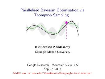
Parallelised Bayesian Optimisation via Thompson Sampling Kirthevasan Kandasamy Akshay Jeff Barnab´ as Krishnamurthy Schneider P´ oczos AISTATS 2018
Black-box Optimisation Expensive Blackbox Function Examples: - Hyper-parameter T uning - ML estimation in Astrophysics - Optimal policy in Autonomous Driving 1/15
Black-box Optimisation f : X → R is an expensive, black-box, noisy function. f ( x ) x 2/15
Black-box Optimisation f : X → R is an expensive, black-box, noisy function. f ( x ) x 2/15
Black-box Optimisation f : X → R is an expensive, black-box, noisy function. Let x ⋆ = argmax x f ( x ). f ( x ) f ( x ∗ ) x ∗ x 2/15
Black-box Optimisation f : X → R is an expensive, black-box, noisy function. Let x ⋆ = argmax x f ( x ). f ( x ) f ( x ∗ ) x ∗ x Simple Regret after n evaluations SR( n ) = f ( x ⋆ ) − max t =1 ,..., n f ( x t ) . 2/15
Gaussian Processes ( GP ) GP ( µ, κ ): A distribution over functions from X to R . 3/15
Gaussian Processes ( GP ) GP ( µ, κ ): A distribution over functions from X to R . Functions with no observations f ( x ) x 3/15
Gaussian Processes ( GP ) GP ( µ, κ ): A distribution over functions from X to R . Prior GP f ( x ) x 3/15
Gaussian Processes ( GP ) GP ( µ, κ ): A distribution over functions from X to R . Observations f ( x ) x 3/15
Gaussian Processes ( GP ) GP ( µ, κ ): A distribution over functions from X to R . Posterior GP given observations f ( x ) x 3/15
Gaussian Processes ( GP ) GP ( µ, κ ): A distribution over functions from X to R . Posterior GP given observations f ( x ) x After t observations, f ( x ) ∼ N ( µ t ( x ) , σ 2 t ( x ) ). 3/15
Gaussian Process Bandit (Bayesian) Optimisation Model f ∼ GP ( 0 , κ ). Several criteria for picking next point: GP-UCB (Srinivas et al. 2010) , GP-EI (Mockus & Mockus, 1991) . f ( x ) x 4/15
Gaussian Process Bandit (Bayesian) Optimisation Model f ∼ GP ( 0 , κ ). Several criteria for picking next point: GP-UCB (Srinivas et al. 2010) , GP-EI (Mockus & Mockus, 1991) . f ( x ) x 1) Compute posterior GP . 4/15
Gaussian Process Bandit (Bayesian) Optimisation Model f ∼ GP ( 0 , κ ). Several criteria for picking next point: GP-UCB (Srinivas et al. 2010) , GP-EI (Mockus & Mockus, 1991) . ϕ t = µ t − 1 + β 1 / 2 f ( x ) σ t − 1 t x 1) Compute posterior GP . 2) Construct acquisition ϕ t . 4/15
Gaussian Process Bandit (Bayesian) Optimisation Model f ∼ GP ( 0 , κ ). Several criteria for picking next point: GP-UCB (Srinivas et al. 2010) , GP-EI (Mockus & Mockus, 1991) . ϕ t = µ t − 1 + β 1 / 2 f ( x ) σ t − 1 t x t x 1) Compute posterior GP . 2) Construct acquisition ϕ t . 3) Choose x t = argmax x ϕ t ( x ). 4/15
Gaussian Process Bandit (Bayesian) Optimisation Model f ∼ GP ( 0 , κ ). Several criteria for picking next point: GP-UCB (Srinivas et al. 2010) , GP-EI (Mockus & Mockus, 1991) . ϕ t = µ t − 1 + β 1 / 2 f ( x ) σ t − 1 t x t x 1) Compute posterior GP . 2) Construct acquisition ϕ t . 3) Choose x t = argmax x ϕ t ( x ). 4) Evaluate f at x t . 4/15
This work: Parallel Evaluations Sequential evaluations with one worker 5/15
This work: Parallel Evaluations Sequential evaluations with one worker Parallel evaluations with M workers (Asynchronous) 5/15
This work: Parallel Evaluations Sequential evaluations with one worker Parallel evaluations with M workers (Asynchronous) Parallel evaluations with M workers (Synchronous) 5/15
This work: Parallel Evaluations Sequential evaluations with one worker j th job has feedback from all previous j − 1 evaluations. Parallel evaluations with M workers (Asynchronous) j th job missing feedback from exactly M − 1 evaluations. Parallel evaluations with M workers (Synchronous) j th job missing feedback from ≤ M − 1 evaluations. 5/15
Challenges in parallel BO: encouraging diversity Direct application of UCB in the synchronous setting . . . ϕ t = µ t − 1 + β 1 / 2 f ( x ) σ t − 1 t x t 1 x - First worker: maximise acquisition, x t 1 = argmax ϕ t ( x ). 6/15
Challenges in parallel BO: encouraging diversity Direct application of UCB in the synchronous setting . . . ϕ t = µ t − 1 + β 1 / 2 f ( x ) σ t − 1 t x t 2 = x t 1 x - First worker: maximise acquisition, x t 1 = argmax ϕ t ( x ). - Second worker: acquisition is the same! x t 1 = x t 2 6/15
Challenges in parallel BO: encouraging diversity Direct application of UCB in the synchronous setting . . . ϕ t = µ t − 1 + β 1 / 2 f ( x ) σ t − 1 t x t 2 = x t 1 x - First worker: maximise acquisition, x t 1 = argmax ϕ t ( x ). - Second worker: acquisition is the same! x t 1 = x t 2 - x t 1 = x t 2 = · · · = x tM . 6/15
Challenges in parallel BO: encouraging diversity Direct application of UCB in the synchronous setting . . . ϕ t = µ t − 1 + β 1 / 2 f ( x ) σ t − 1 t x t 2 = x t 1 x - First worker: maximise acquisition, x t 1 = argmax ϕ t ( x ). - Second worker: acquisition is the same! x t 1 = x t 2 - x t 1 = x t 2 = · · · = x tM . Direct application of popular (deterministic) strategies, e.g. GP-UCB , GP-EI , etc. do not work. Need to “encourage diversity”. 6/15
Challenges in parallel BO: encouraging diversity ◮ Add hallucinated observations. (Ginsbourger et al. 2011, Janusevkis et al. 2012) ◮ Optimise an acquisition over X M (e.g. M -product UCB). ( Wang et al 2016, Wu & Frazier 2017 ) ◮ Resort to heuristics, typically requires additional hyper-parameters and/or computational routines. (Contal et al. 2013, Gonzalez et al. 2015, Shah & Ghahramani 2015, Wang et al. 2017, Wang et al. 2018) 7/15
Challenges in parallel BO: encouraging diversity ◮ Add hallucinated observations. (Ginsbourger et al. 2011, Janusevkis et al. 2012) ◮ Optimise an acquisition over X M (e.g. M -product UCB). ( Wang et al 2016, Wu & Frazier 2017 ) ◮ Resort to heuristics, typically requires additional hyper-parameters and/or computational routines. (Contal et al. 2013, Gonzalez et al. 2015, Shah & Ghahramani 2015, Wang et al. 2017, Wang et al. 2018) Our Approach: Based on Thompson sampling (Thompson, 1933) . ◮ Conceptually simple: does not require explicit diversity strategies. 7/15
Challenges in parallel BO: encouraging diversity ◮ Add hallucinated observations. (Ginsbourger et al. 2011, Janusevkis et al. 2012) ◮ Optimise an acquisition over X M (e.g. M -product UCB). ( Wang et al 2016, Wu & Frazier 2017 ) ◮ Resort to heuristics, typically requires additional hyper-parameters and/or computational routines. (Contal et al. 2013, Gonzalez et al. 2015, Shah & Ghahramani 2015, Wang et al. 2017, Wang et al. 2018) Our Approach: Based on Thompson sampling (Thompson, 1933) . ◮ Conceptually simple: does not require explicit diversity strategies. ◮ Asynchronicity ◮ Theoretical guarantees 7/15
GP Optimisation with Thompson Sampling (Thompson, 1933) f ( x ) x 8/15
GP Optimisation with Thompson Sampling (Thompson, 1933) f ( x ) x 1) Construct posterior GP . 8/15
GP Optimisation with Thompson Sampling (Thompson, 1933) f ( x ) x 1) Construct posterior GP . 2) Draw sample g from posterior. 8/15
GP Optimisation with Thompson Sampling (Thompson, 1933) f ( x ) x t x 1) Construct posterior GP . 2) Draw sample g from posterior. 3) Choose x t = argmax x g ( x ). 8/15
GP Optimisation with Thompson Sampling (Thompson, 1933) f ( x ) x t x 1) Construct posterior GP . 2) Draw sample g from posterior. 3) Choose x t = argmax x g ( x ). 4) Evaluate f at x t . 8/15
GP Optimisation with Thompson Sampling (Thompson, 1933) f ( x ) x t x 1) Construct posterior GP . 2) Draw sample g from posterior. 3) Choose x t = argmax x g ( x ). 4) Evaluate f at x t . Take-home message: In parallel settings, direct application of sequential TS algorithm works. Inherent randomness adds sufficient diversity when managing M workers. 8/15
Parallelised Thompson Sampling Asynchronous: asyTS At any given time, 1. ( x ′ , y ′ ) ← Wait for a worker to finish. 2. Compute posterior GP . 3. Draw a sample g ∼ GP . 4. Re-deploy worker at argmax g . 9/15
Parallelised Thompson Sampling Synchronous: synTS Asynchronous: asyTS At any given time, At any given time, m ) } M 1. ( x ′ , y ′ ) ← Wait for 1. { ( x ′ m , y ′ m =1 ← Wait for a worker to finish. all workers to finish. 2. Compute posterior GP . 2. Compute posterior GP . 3. Draw a sample g ∼ GP . 3. Draw M samples g m ∼ GP , ∀ m . 4. Re-deploy worker at 4. Re-deploy worker m at argmax g m , ∀ m . argmax g . 9/15
Parallelised Thompson Sampling Synchronous: synTS Asynchronous: asyTS At any given time, At any given time, m ) } M 1. ( x ′ , y ′ ) ← Wait for 1. { ( x ′ m , y ′ m =1 ← Wait for a worker to finish. all workers to finish. 2. Compute posterior GP . 2. Compute posterior GP . 3. Draw a sample g ∼ GP . 3. Draw M samples g m ∼ GP , ∀ m . 4. Re-deploy worker at 4. Re-deploy worker m at argmax g m , ∀ m . argmax g . Parallel TS in prior work: (Osband et al. 2016, Israelsen et al. 2016, Hernandez-Lobato et al. 2017) 9/15
Simple Regret in Parallel Settings Simple regret after n evaluations , SR( n ) = f ( x ⋆ ) − max t =1 ,..., n f ( x t ) . n ← # completed evaluations by all workers. 10/15
Recommend
More recommend
Explore More Topics
Stay informed with curated content and fresh updates.
