Parallel Tomographic Reconstruction Where Introduction - PowerPoint PPT Presentation
Parallel Tomographic Reconstruction Where Introduction Combinatorics Meets Geometry X-rays Sparse matrix Exact (S) MondriaanOpt MP Rob H. Bisseling Results Heuristic (M) Mathematical Institute, Utrecht University Medium-grain
Parallel Tomographic Reconstruction – Where Introduction Combinatorics Meets Geometry X-rays Sparse matrix Exact (S) MondriaanOpt MP Rob H. Bisseling Results Heuristic (M) Mathematical Institute, Utrecht University Medium-grain Iterative refinement Results SIAM Conf. on Parallel Processing for Scientific Computing Geometric (L) Bipartitioning SIAM Workshop on Combinatorial Scientific Computing High resolution Results Seattle, February 12, 2020 Conclusion and outlook (XL) Thanks to: Jan-Willem Buurlage, Timon Knigge, Dani¨ el Pelt 1
Introduction: computed tomography X-rays Sparse tomography matrix Small problems: exact sparse matrix partitioning Introduction X-rays Branch-and-bound bipartitioner MondriaanOpt Sparse matrix Improved bipartitioner MP Exact (S) MondriaanOpt Database of optimally bipartitioned matrices MP Results Medium-size problems: heuristic sparse matrix partitioning Heuristic (M) Medium-grain Medium-grain partitioning Iterative refinement Results Iterative refinement: chicken-or-egg Geometric (L) How far from optimal? Bipartitioning High resolution Large tomography problems: geometric data partitioning Results Conclusion and Bipartitioning outlook (XL) High resolution Parallel speedup on GPUs Conclusion and outlook 2
Mondriaan sparse matrix partitioning Introduction X-rays Sparse matrix Exact (S) MondriaanOpt MP Results Heuristic (M) Medium-grain Iterative refinement Results Composition with red, Geometric (L) 4-way partitioning of Bipartitioning yellow, blue, and black High resolution matrix impcol b Results Piet Mondriaan, 1921 Conclusion and outlook (XL) ◮ Mondriaan is an open-source software package for sparse matrix partitioning. ◮ Version 1.0, May 2002. Version 4.2.1, August 2019. 3
Introduction X-rays Sparse matrix Exact (S) Introduction: MondriaanOpt MP Results computed tomography Heuristic (M) Medium-grain Iterative refinement Results Geometric (L) Bipartitioning High resolution Results Conclusion and outlook (XL) 4
Tomography setup Introduction X-rays Sparse matrix Exact (S) MondriaanOpt MP Results Heuristic (M) Medium-grain Iterative refinement Results Geometric (L) Bipartitioning High resolution Results Conclusion and outlook (XL) ◮ One projection from the point source to a detector. ◮ 7 X-rays penetrating the object. 5
Flexible CT scanner at CWI Amsterdam Introduction X-rays Sparse matrix Exact (S) MondriaanOpt MP Results Heuristic (M) Medium-grain Iterative refinement Results Geometric (L) Bipartitioning High resolution Results Conclusion and outlook (XL) 6
Modern art object in the scanner Introduction X-rays Sparse matrix Exact (S) MondriaanOpt MP Results Heuristic (M) Medium-grain Iterative refinement Results Geometric (L) Bipartitioning High resolution Results Conclusion and outlook (XL) ◮ Nel Haringa and Fred Olijve: Homage to De Stijl, 2004. Acrylic and perspex. 7
One projection of the art object Introduction X-rays Sparse matrix Exact (S) MondriaanOpt MP Results Heuristic (M) Medium-grain Iterative refinement Results Geometric (L) Bipartitioning High resolution Results Conclusion and outlook (XL) 8
Helical cone beam Introduction X-rays Sparse matrix Exact (S) MondriaanOpt MP Results Heuristic (M) Medium-grain Iterative refinement Results Geometric (L) Bipartitioning High resolution Results Conclusion and outlook (XL) ◮ Scanner and detector move in a circle around the object. ◮ Object (or scanner) moves along the rotation axis. 9
Acquisition geometries and their application field Introduction X-rays Sparse matrix Exact (S) MondriaanOpt ◮ Helical cone beam: medical imaging, rock samples MP Results ◮ Parallel beam: electron microscopy, synchrotrons Heuristic (M) ◮ Laminography: inspection of flat objects Medium-grain Iterative refinement Results ◮ Tomosynthesis: mammography, airport security screening Geometric (L) Bipartitioning High resolution Results Conclusion and outlook (XL) 10
Solving a sparse linear system 4 projections 5 × 5 detector pixels Introduction 5 × 5 × 5 object voxels X-rays Sparse matrix Exact (S) m = 100, n = 125 MondriaanOpt MP 1394 nonzeros Results Heuristic (M) Medium-grain n − 1 Iterative refinement Results � b i = 0 ≤ i < m . a ij x j , Geometric (L) j =0 Bipartitioning High resolution Results ◮ a ij is the weight of ray i in voxel j , Conclusion and outlook (XL) ◮ x j is the density of voxel j , ◮ b i is the detector measurement for ray i . ◮ Not every ray hits every voxel: the system is sparse. ◮ Usually m < n : the system is underdetermined. 11
Simultaneous Iterative Reconstruction Technique Introduction ◮ SIRT repeatedly multiplies the sparse matrices A and A T X-rays Sparse matrix with a vector until convergence. Exact (S) MondriaanOpt ◮ For low resolutions, A is small and it can be stored. MP Results ◮ However, for a high resolution of 4000 3 = 64 × 10 9 voxels, Heuristic (M) A has 256 × 10 12 nonzeros, so we have Petabytes of data. Medium-grain Iterative refinement Results ◮ For large problem sizes, implementations are matrix-free: Geometric (L) A is too big to store, and too big to partition by a Bipartitioning High resolution combinatorial method. Results ◮ We can regenerate the matrix easily row by row. Conclusion and outlook (XL) 12
Introduction X-rays Sparse matrix Exact (S) Small problems: MondriaanOpt MP Results exact sparse matrix partitioning Heuristic (M) Medium-grain Iterative refinement Results Geometric (L) Bipartitioning High resolution Results Conclusion and outlook (XL) 13
Parallel sparse matrix–vector multiplication u := A v Introduction X-rays 2 1 1 4 3 v T Sparse matrix Exact (S) MondriaanOpt MP Results 6 3 1 Heuristic (M) Medium-grain 9 4 1 Iterative refinement Results 22 5 9 2 Geometric (L) Bipartitioning High resolution 41 6 5 3 Results Conclusion and 64 5 8 9 outlook (XL) u A 14
Optimal bipartitioning by MondriaanOpt Introduction 7 × 7 matrix b1 ss X-rays nz ( A ) = 15, V = 3 Sparse matrix Exact (S) MondriaanOpt MP Results Heuristic (M) ◮ Benchmark p = 2 because heuristic partitioners are often Medium-grain Iterative refinement based on recursive bipartitioning. Results Geometric (L) ◮ Problem p = 2 is easier to solve than p > 2. Bipartitioning ◮ Load balance criterion is High resolution Results � nz ( A ) � Conclusion and nz ( A i ) ≤ (1 + ε ) i = 0 , 1 , , outlook (XL) 2 where ε ∈ [0 , 1) is the allowed load imbalance fraction. D. M. Pelt and R. H. Bisseling, “An exact algorithm for sparse matrix bipartitioning”, JPDC 85 (2015) pp. 79–90. 15
Branch-and-bound method Introduction X-rays Evening – the red tree Sparse matrix Piet Mondriaan, 1908 Exact (S) MondriaanOpt MP Results Heuristic (M) Medium-grain Iterative refinement Results ◮ Construct a ternary tree representing all possible solutions Geometric (L) ◮ Every node in the tree has 3 branches, representing a Bipartitioning High resolution choice for a matrix row or column: Results • completely assigned to processor P (0) Conclusion and outlook (XL) • completely assigned to processor P (1) • cut: assigned to processors P (0) and P (1) ◮ The tree is pruned by using lower bounds on the communication volume or number of nonzeros 16
Packing bound on communication volume 0 1 - - - c Introduction X-rays 0 Sparse matrix - Exact (S) - MondriaanOpt - MP Results Heuristic (M) Medium-grain Iterative refinement Results ◮ Columns 3, 4, 5 have been partially assigned to P (0). Geometric (L) ◮ They can only be completely assigned to P (0) or cut. Bipartitioning High resolution ◮ For perfect load balance ( ε = 0), we can pack at most 2 Results Conclusion and more red nonzeros into P (0). outlook (XL) ◮ Thus we have to cut column 3, and one more column, giving 2 communications. ◮ We call the resulting lower bound a packing bound. 17
From sparse matrix to bipartite graph − − 1 Row 0 Col 0 Introduction X-rays Sparse matrix − Exact (S) MondriaanOpt MP − Row 1 Col 1 Results Heuristic (M) Medium-grain Iterative refinement 0 Results Geometric (L) Bipartitioning Row 2 Col 2 High resolution Results Row 2 has been assigned to part 0 and column 1 to part 1. Conclusion and outlook (XL) T. E. Knigge and R. H. Bisseling, “An improved exact algorithm and an NP-completeness proof for sparse matrix bipartitioning”, submitted. https://github.com/TimonKnigge/matrix-partitioner 18
Flow bound on communication − 1 c Row 0 Col 0 Introduction X-rays Sparse matrix − Exact (S) MondriaanOpt MP − Row 1 Col 1 Results Heuristic (M) Medium-grain 0 Iterative refinement Results Geometric (L) Bipartitioning Row 2 Col 2 High resolution Results Along the path from row 2 to column 1, at least one row or Conclusion and outlook (XL) column must be cut. We can model the problem with multiple paths as a maximum-flow problem. 19
Recommend
More recommend
Explore More Topics
Stay informed with curated content and fresh updates.
