2D Fan Beam Reconstruction 3D Cone Beam Reconstruction Mario - PDF document

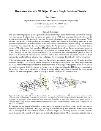
2D Fan Beam Reconstruction 3D Cone Beam Reconstruction Mario Koerner March 17, 2006 1 2D Fan Beam Reconstruction Two-dimensional objects can be reconstructed from projections that were acquired using parallel projection rays. A practical algorithm for doing so is the Filtered Backprojection (FBP). It consists of 2 steps: 1. filtering the projection data with a high-pass filter 2. backprojecting the filtered projections over the object domain The drawback of this simple parallel projection geometry is that it requires a complex mechanical system to get the required data. To acquire a single projection image, it is nec- essary to move the source-detector pair along parallel lines and scan the projection rays one by one. Of course, this is also very time consuming. A much faster method of data collection would be to rotate the radiation source around the object an sample a complete fan of projection on the detector at each position. A com- parison of the two geometries is shown in Figure 1. 1.1 Equiangular rays First we will assume that the rays of the fan are sampled in equiangular intervals, i.e. they are measured at equidistant intervals on a circular detector. The rotation angle of the source with respect to the y-axis of the coordinate system will be denoted by β , the angle between a specific projection ray and the central ray of the fan will be denoted by γ . The FBP integral for parallel beams can be written (using polar coordinates for points in object space) as follows: � 2 π � t m f ( x, y ) = 1 P θ ( t ) h ( x cos θ + y sin θ − t ) dtdθ (1) 2 0 − t m To use this formula for the fan beam case, we need to know, which projection ray of a parallel beam data set corresponds to each projection ray in the collected fan beam data set. Figure 2 shows the acquisition parameters for the projection ray SA in the parallel beam dataset ( θ , t) and the parameters in the fan beam data set ( β , γ ). The transformation between these two is given by θ = β + γ (2) t = D sin γ (3) 1

Figure 1: Comparison of parallel beam and fan beam geometry Figure 2: A projection ray in a fan beam projection and in a parallel projection (from [Kak]) 2

Applying this transformation to the FBP integral for the parallel beam case and doing some further conversions leads to a formula that can be interpreted as a weighted FBP. A detailed derivation can be found in [Kak]. � 2 π � γ m 1 R β ( γ ) D cos γg ( γ ′ − γ ) dγdβ f ( x, y ) = (4) L 2 0 − γ m with γ ′ identifying the projection ray in projection β , where the point (x,y) lies on. x cos β + y sin β γ ′ ( x, y, β ) = tan − 1 (5) D + x sin β − y cos β So the FBP algorithm for reconstructing a 2D object from fan beam projections consists of the following 3 steps: 1. Pre-weight the projection data according to R ′ β ( γ ) = R β ( γ ) D cos γ (6) 2. Filter the projections using the discrete filtering kernel g ( γ ) = 1 2( γ sin γ ) 2 h ( γ ) (7) where h( γ ) is the ramp filter from the parallel beam case. 3. Perform a weighted backprojection of the filtered projections along the fan with the distance L from the point to be reconstructed to the source as weight. ( D + x sin β − y cos β ) 2 + ( x cos β + y sin β ) 2 � L ( x, y, β ) = (8) 1.2 Equally spaced collinear detectors In the previous section we assumed the projection data to be sampled in equiangular inter- vals on a circular detector. However, e.g. C-arm systems use planar detectors to measure projections, because their primary use is the acquisition of classical X-ray images. Similar to the case of equiangular fan beams, a coordinate transformation can be applied to the FBP integral to transform the acquisition parameters ( β , s) to the parallel case. As seen in Figure 3 they are related to ( θ , t) using θ = β + γ = β + tan − 1 s (9) D sD t = s cos γ = (10) √ D 2 + s 2 The resulting FBP formula is: � 2 π � ∞ 1 D D 2 + s 2 g ( s ′ − s ) dsdβ f ( x, y ) = R β ( s ) (11) √ U 2 0 −∞ The algorithm consists of the steps 3

Figure 3: A projection ray in a fan beam projection and in a parallel projection (from [Kak]) 1. Pre-weight the projection data according to D R ′ β ( s ) = R β ( s ) (12) √ D 2 + s 2 Note that the weighting factor can be interpreted as the cosine of the angle between the considered projection ray and the central ray of the current projection. 2. Filter the projections using the discrete filtering kernel g ( s ) = 1 2 h ( s ) (13) where h( γ ) is the ramp filter from the parallel beam case. 3. Perform a weighted backprojection of the filtered projections along the fan with the weight U, which is the ratio between the parallel projection of point (x,y) onto the central ray (SP in figure 4) and the source center distance D. U ( x, y, β ) = D + x sin β − y cos β (14) D 4

Figure 4: The weighting factor U for a pixel (x,y) (denoted in polar coordinates here) is the ration between SP and D (from [Kak]) 5

Figure 5: Shortscan measurement 2 Short Scan Reconstruction Not in all technical environments it is possible to rotate the radiation source and the detector around the object by full 360 degrees. For the parallel case, it is easy to see, that a rotation over 180 degrees is sufficient to measure all data required for reconstruction, because 2 projections with an offset of 180 degree are mirror images of each other. Unfortunately this is not true for the fan beam case. If the rotation only goes over 180 degrees, some projection rays are missing in the acquired data set while others are measured twice. To acquire a complete data set, the overall rotation needs to be extended to 180 ◦ +2 γ m , but this adds even more redundancy. Figure 5 shows the sinogram of the measurement transformed into the β/γ space. Each point represents a projection ray that is included in the measurement. The shaped areas mark the regions, where 2 measurements exist: F corresponds to C, D corresponds to B and E corresponds to A. One could think, that the redundancy problem can be solved by wiping out the data in the triangle ABC. Although this would remove the redundancy, the sharp edge between non-redundant and the wiped out redundant data introduces high frequencies, which are enhanced by the following filtering operation with the ramp filter. This leads to heavy arti- facts in the reconstruction result. 2.1 Parker weighting A better way to handle the redundancy is to construct a smooth (continuously differentiable) window function that properly weights the data. The Parker window function is such a function: sin 2 (45 ◦ β  γ m + γ ) : on ABC  sin 2 (45 ◦ 180 ◦ +2 γ m − β w β ( γ ) = ) : on DEF (15) γ m − γ  1 : elsewhere This function is zero on the lines AB and EF, one on the lines AC and DE and has contin- uous partial derivatives over the complete region. 6

Weighting the projection data with this window function before starting the FBP leads to good reconstruction results. 2.2 Parallel rebinning Instead of using Parker weighting and the FBP for fan beam projections, a parallel projection set can be generated using R β ( γ ) = P β + γ ( D sin γ ) (16) This step is called rebinning. Unfortunately this is not just a rearrangement of data. An interpolation is required to transform the data set. Redundant input data is just discarded. The actual reconstruction is done by applying the FBP algorithm to the generated data for rotation angles between 0 and 180 degrees. 7

Figure 6: Cone Beam geometry 3 3D Cone Beam Reconstruction As for 2D objects it is cumbersome to collect each parallel line integral separately, this also holds for 3D objects that are scanned slice by slice. If slices of a 3D object are measured, the reconstruction can be done using 2D methods and putting together all slices at the end. Data acquisition would be much faster, if we could use a bunch of fan projections (form- ing a cone, see figure 6) and rotate around the object just once. The problem is, that this configuration does not allow exact reconstruction, meaning that there will always be an er- ror, no matter how many projections are used and how high the detector resolution is. There exist approximate methods, one of them is the Feldkamp algorithm, which was developed by Feldkamp, Davis and Kress in 1984. 3.1 The Feldkamp algorithm The Feldkamp algorithm is very similar to the 2D FBP for fan beam projections. Due to its simplicity it is widely spread in many practical applications. 3 Steps are required to perform the reconstruction: 1. Pre-weight the projection rays according to their position within the 3D cone: D R ′ β ( a, b ) = R β ( a, b ) (17) √ D 2 + a 2 + b 2 Note that the weighting factor can be interpreted as the cosine of the angle between the considered projection ray and the central ray of the current projection. 2. Filter the projections along horizontal detector lines using the same discrete filtering kernel as on 2D fan beam data g ( s ) = 1 2 h ( s ) (18) Q β ( a, b ) = R ′ β ( a, b ) ∗ g ( a ) (19) 8

3. Perform a weighted backprojection of the filtered projections along the cone with the same weighting factor U as in the 2D fan beam case. 4 Literature references [Kak ] A. C. Kak and Malcolm Slaney, Principles of Computerized Tomographic Imaging. Society of Industrial and Applied Mathematics, 2001 [Tur ] Henrik Turbell, Cone-Beam Reconstruction using Filtered Backprojection. Disserta- tion, Linkping Studies in Science and Technology, 2001 9