Paper reviews Thorough summary in your own words Main - PDF document

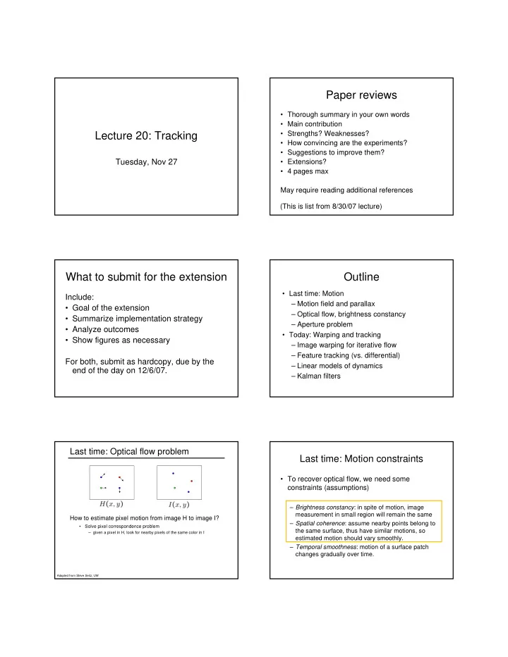
Paper reviews • Thorough summary in your own words • Main contribution • Strengths? Weaknesses? Lecture 20: Tracking • How convincing are the experiments? • Suggestions to improve them? Tuesday, Nov 27 • Extensions? • 4 pages max May require reading additional references (This is list from 8/30/07 lecture) What to submit for the extension Outline • Last time: Motion Include: – Motion field and parallax • Goal of the extension – Optical flow, brightness constancy • Summarize implementation strategy – Aperture problem • Analyze outcomes • Today: Warping and tracking • Show figures as necessary – Image warping for iterative flow – Feature tracking (vs. differential) For both, submit as hardcopy, due by the – Linear models of dynamics end of the day on 12/6/07. – Kalman filters Last time: Optical flow problem Last time: Motion constraints • To recover optical flow, we need some constraints (assumptions) – Brightness constancy : in spite of motion, image measurement in small region will remain the same How to estimate pixel motion from image H to image I? – Spatial coherence : assume nearby points belong to • Solve pixel correspondence problem the same surface, thus have similar motions, so – given a pixel in H, look for nearby pixels of the same color in I estimated motion should vary smoothly. – Temporal smoothness : motion of a surface patch changes gradually over time. Adapted from Steve Seitz, UW

Last time: Brightness constancy equation Last time: Aperture problem • Brightness constancy equation: single equation, dI two unknowns; infinitely many solutions. = Total derivative: x and y are 0 also functions of time t dt spatial gradients: how ∂ ∂ ∂ I dx I dy I image varies in x or y • Can only compute projection of actual flow = + + direction for fixed time ∂ ∂ ∂ vector [ u , v ] in the direction of the image gradient, x dt y dt t temporal gradient : how that is, in the direction normal to the image edge. image varies in time for fixed position – Flow component in gradient direction determined Rewritten: temporal derivatives , – Flow component parallel to edge unknown. u and v : rate of change in x and y Last time: Solving the aperture problem Last time: Lucas-Kanade flow How to get more equations for a pixel? Prob: we have more equations than unknowns • Basic idea: impose additional constraints – most common is to assume that the flow field is smooth locally – one method: pretend the pixel’s neighbors have the same (u,v) Solution: solve least squares problem » If we use a 5x5 window, that gives us 25 equations per pixel! • minimum least squares solution given by solution (in d) of: • The summations are over all pixels in the K x K window • This technique was first proposed by Lucas & Kanade (1981) Adapted from Steve Seitz, UW Slide by Steve Seitz, UW Image warping Difficulties • When will this flow computation fail? – If brightness constancy is not satisfied T ( x,y ) • E.g., occlusions, illumination change… y y’ – If the motion is not small x x’ f ( x,y ) g ( x’,y’ ) • derivative estimates poor – If points within window neighborhood do not move together Given a coordinate transform and a source image • E.g., if window size is too large f ( x,y ), how do we compute a transformed image g(x’,y’) = f ( T ( x,y ))? Slide from Alyosha Efros, CMU

Inverse warping Inverse warping T -1 ( x,y ) T -1 ( x,y ) y y’ y y’ x x x’ x x x’ f ( x,y ) g ( x’,y’ ) f ( x,y ) g ( x’,y’ ) Get each pixel g ( x’,y’ ) from its corresponding location Get each pixel g ( x’,y’ ) from its corresponding location ( x,y ) = T -1 ( x’,y’ ) in the first image ( x,y ) = T -1 ( x’,y’ ) in the first image Q: what if pixel comes from “between” two pixels? Q: what if pixel comes from “between” two pixels? A: Interpolate color value from neighbors – nearest neighbor, bilinear… Slide from Alyosha Efros, CMU Slide from Alyosha Efros, CMU Bilinear interpolation Iterative flow computation Sampling at f(x,y): To iteratively refine flow estimates, repeat until warped version of first image very close to second image: • compute flow vector [u, v] • warp image toward the other using estimated flow field Slide from Alyosha Efros, CMU Figure from Martial Hebert, CMU Feature Detection Tracking features Feature tracking • Compute optical flow for that feature for each consecutive frame pair When will this go wrong? • Occlusions—feature may disappear – need mechanism for deleting, adding new features • Changes in shape, orientation – allow the feature to deform • Changes in color • Large motions Adapted from Steve Seitz, UW

Handling large motions Derivative-based flow computation requires small motion. • If the motion is much more than a pixel, use discrete search instead • For a discrete matching search, what are the tradeoffs of the chosen search window size? • Given feature window W in H, find best matching window in I • Minimize sum squared difference (SSD) of pixels in window • Solve by doing a search over a specified range of (u,v) values – this (u,v) range defines the search window Adapted from Steve Seitz, UW Summary: Motion field estimation • Differential techniques – optical flow: use spatial and temporal variation of image brightness at all pixels • Tracking with features: where should the – assumes we can approximate motion field by search window be placed? constant velocity within small region of image plane – Near match at previous frame • Feature matching techniques – More generally, according to expected – estimate disparity of special points (easily dynamics of the object tracked features) between frames – sparse Think of stereo matching: same as estimating motion if we have two close views or two frames close in time. Detection vs. tracking Detection vs. tracking … … t=1 t=2 t=20 t=21 Detection: We detect the object independently in each frame and can record its position over time, e.g., based on blob’s centroid or detection window coordinates

Detection vs. tracking Goal of tracking • Have a model of expected motion • Given that, predict where objects will occur in next frame, even before seeing the image … • Intent: – do less work looking for the object, restrict search – improved estimates since measurement noise Tracking with dynamics : We use image measurements to estimate position of object, but tempered by trajectory smoothness also incorporate position predicted by dynamics, i.e., our expectation of object’s motion pattern. Example of Bayesian Inference General assumptions Cost model Sensor model cost(fast walk | staircase) = $1,000 p(image | staircase) = 0.7 p(staircase) Slow cost(fast walk | no staircase) = $0 p(image | no staircase) = 0.2 • Expect motion to be continuous, so we can cost(slow+sense) = $1 Down! = 0.28 Environment prior predict based on previous trajectories p(staircase) = 0.1 – Camera is not moving instantly from viewpoint Decision Theory Bayesian inference E[cost(fast walk)] = $1,000 • 0.28 = $280 p(staircase | image) to viewpoint p(image | staircasse) p(staircase) E[cost(slow+sense)] = $1 = p(im | stair) p(stair) + p(im | no stair) p(no stair) – Objects do not disappear and reappear in = 0.7 • 0.1 / (0.7 • 0.1 + 0.2 • 0.9) = 0.28 different places in the scene ? – Gradual change in pose between camera and scene • Able to model the motion Slide by Sebastian Thrun and Jana Košecká, Stanford University Tracking as inference: Bayes Filters Idea of recursive estimation � Hidden state x t – The unknown true parameters – E.g., actual position of the person we are tracking � Measurement y t – Our noisy observation of the state – E.g., detected blob’s centroid Note temporary change of notation: state � Can we calculate p ( x t | y 1 , y 2 , …, y t ) ? is a , and measurement at time step i is x i . – Want to recover the state from the observed measurements Adapted from Cornelia Fermüller, UMD.

Idea of recursive estimation Idea of recursive estimation Adapted from Cornelia Fermüller, UMD. Adapted from Cornelia Fermüller, UMD. Idea of recursive estimation Idea of recursive estimation Adapted from Cornelia Fermüller, UMD. Adapted from Cornelia Fermüller, UMD. Idea of recursive estimation Idea of recursive estimation Adapted from Cornelia Fermüller, UMD. Adapted from Cornelia Fermüller, UMD.

Inference for tracking Idea of recursive estimation • Recursive process: – Assume we have initial prior that predicts state in absence of any evidence: P( X 0 ) – At the first frame , correct this given the value of Y 0 = y 0 – Given corrected estimate for frame t • Predict for frame t+1 • Correct for frame t+1 Adapted from Cornelia Fermüller, UMD. Tracking as inference Assume independences to simplify • Prediction: • Only immediate past state influences current state – Given the measurements we have seen up to this point, what state should we predict? • Measurements at time t only depend on • Correction: the current state – Now given the current measurement, what state should we predict? Base case Induction step: prediction

Induction step: correction Inference for tracking • Goal is then to – choose good model for the prediction and correction distributions – use the updates to compute best estimate of state • Prior to seeing measurement • After seeing the measurement • We stopped here on Tuesday, to be continued on Thursday.