
SLIDE 1
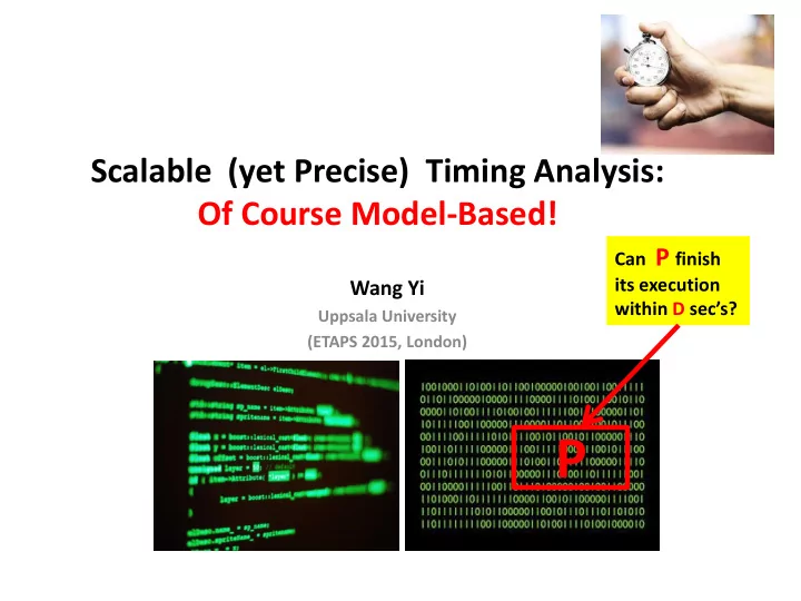
Scalable (yet Precise) Timing Analysis: Of Course Model-Based!
Wang Yi
Uppsala University (ETAPS 2015, London)
P
Can P finish its execution within D sec’s?
P Joint work with my students: Martin Stigge Nan Guan Pontus - - PowerPoint PPT Presentation
Scalable (yet Precise) Timing Analysis: Of Course Model-Based! Can P finish its execution Wang Yi within D secs ? Uppsala University (ETAPS 2015, London) P Joint work with my students: Martin Stigge Nan Guan Pontus Ekberg Jakaria
Scalable (yet Precise) Timing Analysis: Of Course Model-Based!
Wang Yi
Uppsala University (ETAPS 2015, London)
Can P finish its execution within D sec’s?
Nan Guan Martin Stigge Pontus Ekberg Jakaria Abdullah
– for the tractable cases
– for the intractable cases
4
I/O I/O DSP
Input Stream Input Stream BUS
ECU I/O FPGA
Output Stream Output Stream
Event arrivals Event arrivals New events New events
TACAS, Aarhus, April 1995 UPPAAL
Johan Bengtsson Kim Larsen Fredrik Larsson Paul Pettersson
Wang Yi
Photo: Kim Larsen, Aalborg Univ.
Model Checking of # model checkers time
I can’t solve the problem, neither can all these famous Model-Checkers
Analysis “Difficulty” Modeling “Expressiveness” “richness”
Tractable (pseudo-p) Analyzable “Needed” for Interesting features
Scalable Efficient
Decidable Run & Pray
ESWEEK CPSWEEK
ETAPS/FLoC
TACAS RTSS ECRTS RTAS EMSOFT CAV LICS CONCUR ICALP
task3
Sequential Case (WCET Analysis) Concurrent Case (Response Time Analysis)
WCET
WCRT WCRT
Non-deterministic releases
task1 task1 task2
WCRT=WCET
D3 D1 D2
task3
Sequential Case (WCET Analysis) Concurrent Case (Response Time Analysis)
WCRT WCRT
Non-deterministic releases
task1 task2
WCRT=WCET
D3 D1 D2
Wilhelm et al Precision >> 95% [aiT tool from AbsInt]
Modeling for (System-Level) Timing Analysis
11
I/O I/O DSP
Input Stream Input Stream BUS
ECU I/O FPGA
Output Stream Output Stream
– Time Intervals over transition firing
– Delays + untimed models e.g. Milner’s CCS
– finite automata + clock constraints
– Layland and Liu’s periodic tasks, 1973 – The variants of L&L model [RTSS community]
– Delay, Tasking, Run-Time System
(yesterday)
Task automata Timed automata
Task automata UML-RT TCSP
Hybrid Automata ….
Timed Petri Nets
Timed game
A system is a set of periodic tasks each described by two numbers:
Feasibility (i.e. EDF-schedulability): no deadline miss if U ≤ 1 Fixed-priority Schedulability: no deadline miss if U ≤
The well-known Rate-Monotonic Scheduling
Task automata Task automata
ALL these models are “tractable” but have limited expressiveness
[Survey, RTS journal, Martin and Wang, 2015]
[Baruah et al, 1998, 2003, 2010] 57 114
Restrictions of Tree/DAG model
Restrictions of Tree/DAG model
Further extension without crossing the “tractable” borderline?
The Digraph Real-Time Model (DRT)
A B C
10 2 11 25 <5,10> <2,4>
e.g. A has WCET 2 and relative deadline 4
<8,15> Procedure PA “release A” Delay(2); PC Procedure PB “release B”; Delay(25); PA Procedure PC “release C” If “condition” then Delay(10); PA else Delay (11); PB
In Ada Tasking: [Stigge et al, RTAS 2011]
The WCET, deadlines and release delays should be ensured by the Ada run-time system
(any path of the graph is a possible behavior)
Demand bound: (10, 5)
(any path of the graph is a possible behavior)
Demand bound : (28, 6) Demand bound : (10, 5)
(any path of the graph is a possible behavior)
Demand bound : (43, 9) Workload: (28, 6) Workload: (10, 5)
Demand Bounds Function (dbf) Time window (43,9) (28,6) (10,5)
Time dbf
The system workload:
[Stigge et al, RTAS 2011]
[RTAS 2011]
implying deadline miss
Time dbf
Units of work a CPU can compute over time (100%)
Workload
Of course, if the BLUE line is always below the RED, the system should work well without deadline miss!
Time dbf
Units of work a CPU can compute over time (100 %)
Workload
If the utilization (long-term rates of DRT’s) of a system is bounded by a constant c < 1, any deadline miss, if exists, must appear before a pseudo-polynomial upper bound:
Time
Units of work a CPU can compute over time
Workload
Here is the intuition why “Pseudo-P”
D
dbf
D =
1 -
Time dbf
The system workload:
D
– the analysis without considering synchronization is SAFE! – Precise analysis possible with “Combinatorial Refinement”
[Stigge/Wang, ECRTS 2012] Static-priority Schedulability
Models Analysis Complexity
Feasibility i.e. EDF-Schedulability
Static-priority Schedulability
General graphs (Di-graph) Pseudo-P Strongly coNP-complete Trees/DAGs Pseudo-P Strongly coNP-complete Cyclic graphs (GMF) Pseudo-P Strongly coNP-complete Sporadic (L&L, deadline≠period) Pseudo-P Pseudo-P L&L (periodic) Linear Pseudo-P
For systems with utilization bounded by a constant less than 1 (or below 100%) Otherwise Strongly coNP-complete [ECRTS 2015, Pontus Ekberg and Wang Yi]
!! The problem open for 25 years, theoretically interesting !! What can we do?
[ECRTS 2012]
solving “Combinatorial Problems” (for timing analysis, it works very well!)
[TACAS 2015]
Time dbf
The system workload:
D
In general, each component may have a set of behaviors e.g. Paths or traces
Often, we have to check some property guaranteed by all the combinations of individual local behaviors and thus may have to enumerate … (combinatorial explosion)
Any non-leaf node father should be an
(… ... father … …) sat F (... … any son … …) sat F
For instance, the Combination of all roots satisfies the desired property implies that all combinations of the leaves satisfy the same property. (roots) sat F (any leave, any leave, … any leave) sat F
for each DRT
for each DRT
for each DRT
“Code is Art” – Daniel Licata
– it should be as simple as possible but not simpler – it should be as expressive as possible but not more
– Expressive enough to capture Ada tasking – Efficient analysis possible: Pseudo-polynomial
– In particular when local search space can be abstracted & ordered –
– Synchronization and resource sharing – Multiprocessor mapping and scheduling – TIMES++, a new tool based on Digraph, aiming at industrial applications
– Worst-Case Execution Time (WCET) analysis
– “too many input” too many execution paths (difficult to find the worst-case) – hardware features e.g. caches (“the HW state” results in different execution times)
57
– which path leads to the WCET ? – well-known technique by ILP – need to know the timing delay
– Cache Analysis: Is a memory access hit or miss? – other factors like pipeline …
loop bound loop bound loop bound loop bound
– which path leads to the WCET ? – well-known technique by ILP – need to know the timing delay
– Cache Analysis: Is a memory access hit or miss?
– other factors like pipeline …
loop bound loop bound loop bound loop bound
FM AH AH AM AM AH AM FM AH AH AH AM NC NC AH
– which path leads to the WCET ? – well-known technique by ILP – need to know the timing delay
– Cache Analysis: Is a memory access hit or miss?
– other factors like pipeline …
loop bound loop bound loop bound loop bound
2 2 2 10 10 2 10 2 2 2 2 10 10 10 2
[aiT tool from AbsInt] [Survey 2015 wang et al] Wilhelm et al Precision >> 95%
task3
Sequential Case (WCET Analysis) Concurrent Case (Response Time Analysis)
WCRT WCRT
Non-deterministic releases
task1 task2
WCRT=WCET
D3 D1 D2