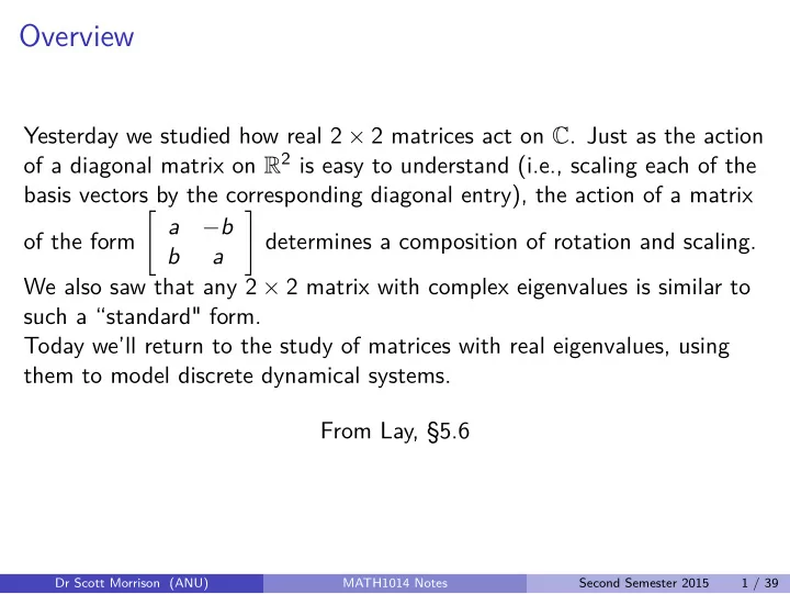
Overview Yesterday we studied how real 2 2 matrices act on C . Just - PowerPoint PPT Presentation

Overview Yesterday we studied how real 2 × 2 matrices act on C . Just as the action of a diagonal matrix on R 2 is easy to understand (i.e., scaling each of the basis vectors by the corresponding diagonal entry), the action of a matrix � � a − b of the form determines a composition of rotation and scaling. b a We also saw that any 2 × 2 matrix with complex eigenvalues is similar to such a “standard" form. Today we’ll return to the study of matrices with real eigenvalues, using them to model discrete dynamical systems. From Lay, §5.6 Dr Scott Morrison (ANU) MATH1014 Notes Second Semester 2015 1 / 39

The main ideas In this section we will look at discrete linear dynamical systems. Dynamics describe the evolution of a system over time, and a discrete system is one where we sample the state of the system at intervals of time, as opposed to studying its continuous behaviour. Finally, these systems are linear because the change from one state to another is described by a vector equation like ( ∗ ) x k +1 = A x k . where A is an n × n matrix and the x k ’s are vectors R n . Dr Scott Morrison (ANU) MATH1014 Notes Second Semester 2015 2 / 39

The main ideas In this section we will look at discrete linear dynamical systems. Dynamics describe the evolution of a system over time, and a discrete system is one where we sample the state of the system at intervals of time, as opposed to studying its continuous behaviour. Finally, these systems are linear because the change from one state to another is described by a vector equation like ( ∗ ) x k +1 = A x k . where A is an n × n matrix and the x k ’s are vectors R n . You should look at the equation above as a recursive relation. Given an initial vector x 0 we obtain a sequence x 0 , x 1 , x 2 , . . . , .. where for every k the vector x k +1 is obtained from the previous vector x k using the relation ( ∗ ). We are generally interested in the long term behaviour of such a system. The applications in Lay focus on ecological problems, but also apply to problems in physics, engineering and many other scientific fields. Dr Scott Morrison (ANU) MATH1014 Notes Second Semester 2015 2 / 39

Initial assumptions We’ll start by describing the circumstances under which our techniques will be effective: The matrix A is diagonalisable. A has n linearly independent eigenvectors v 1 , . . . , v n with corresponding eigenvalues λ 1 , . . . , λ n . The eigenvectors are arranged so that | λ 1 | ≥ | λ 2 | ≥ · · · ≥ | λ n | . Dr Scott Morrison (ANU) MATH1014 Notes Second Semester 2015 3 / 39

Initial assumptions We’ll start by describing the circumstances under which our techniques will be effective: The matrix A is diagonalisable. A has n linearly independent eigenvectors v 1 , . . . , v n with corresponding eigenvalues λ 1 , . . . , λ n . The eigenvectors are arranged so that | λ 1 | ≥ | λ 2 | ≥ · · · ≥ | λ n | . Since { v 1 , . . . , v n } is a basis for R n , any initial vector x 0 can be written x 0 = c 1 v 1 + · · · + c n v n . This eigenvector decomposition of x 0 determines what happens to the sequence { x k } . Dr Scott Morrison (ANU) MATH1014 Notes Second Semester 2015 3 / 39

Since x 0 = c 1 v 1 + · · · + c n v n , we have x 1 = A x 0 = c 1 A v 1 + · · · + c n A v n = c 1 λ 1 v 1 + · · · + c n λ n v n Dr Scott Morrison (ANU) MATH1014 Notes Second Semester 2015 4 / 39

Since x 0 = c 1 v 1 + · · · + c n v n , we have x 1 = A x 0 = c 1 A v 1 + · · · + c n A v n = c 1 λ 1 v 1 + · · · + c n λ n v n x 2 = A x 1 = c 1 λ 1 A v 1 + · · · + c n λ n A v n c 1 ( λ 1 ) 2 v 1 + · · · + c n ( λ n ) 2 v n = and in general, x k = c 1 ( λ 1 ) k v 1 + · · · + c n ( λ n ) k v n (1) We are interested in what happens as k → ∞ . Dr Scott Morrison (ANU) MATH1014 Notes Second Semester 2015 4 / 39

Predator - Prey Systems Example See Example 1, Section 5.6 � � O k The owl and wood rat populations at time k are described by x k = , R k where k is the time in months, O k is the number of owls in the region studied, and R k is the number of rats (measured in thousands). Since owls eat rats, we should expect the population of each species to affect the future population of the other one. The changes in theses populations can be described by the equations: O k +1 = (0 . 5) O k + (0 . 4) R k R k +1 = − p · O k + (1 . 1) R k where p is a positive parameter to be specified. Dr Scott Morrison (ANU) MATH1014 Notes Second Semester 2015 5 / 39

In matrix form this is � � 0 . 5 0 . 4 x k +1 = x k . − p 1 . 1 Dr Scott Morrison (ANU) MATH1014 Notes Second Semester 2015 6 / 39

In matrix form this is � � 0 . 5 0 . 4 x k +1 = x k . − p 1 . 1 Example (Case 1) p = 0 . 104 � � 0 . 5 0 . 4 This gives A = − 0 . 104 1 . 1 According to the book, the eigenvalues for A are λ 1 = 1 . 02 and λ 2 = 0 . 58. Corresponding eigenvectors are, for example, � � � � 10 5 v 1 = , v 2 = . 13 1 Dr Scott Morrison (ANU) MATH1014 Notes Second Semester 2015 6 / 39

An initial population x 0 can be written as x 0 = c 1 v 1 + c 2 v 2 . Then for k ≥ 0, c 1 (1 . 02) k v 1 + c 2 (0 . 58) k v 2 x k = � � � � 10 5 c 1 (1 . 02) k + c 2 (0 . 58) k = 13 1 Dr Scott Morrison (ANU) MATH1014 Notes Second Semester 2015 7 / 39

An initial population x 0 can be written as x 0 = c 1 v 1 + c 2 v 2 . Then for k ≥ 0, c 1 (1 . 02) k v 1 + c 2 (0 . 58) k v 2 x k = � � � � 10 5 c 1 (1 . 02) k + c 2 (0 . 58) k = 13 1 As k → ∞ , (0 . 58) k → 0. Assume c 1 > 0. Then for large k , � � 10 x k ≈ c 1 (1 . 02) k 13 and � � 10 x k +1 ≈ c 1 (1 . 02) k +1 ≈ 1 . 02 x k . 13 Dr Scott Morrison (ANU) MATH1014 Notes Second Semester 2015 7 / 39

The last approximation says that eventually both the population of rats and the population of owls grow by a factor of almost 1.02 per month, a 2% growth rate. The ratio 10 to 13 of the entries in x k remain the same, so for every 10 owls there are 13 thousand rats. Dr Scott Morrison (ANU) MATH1014 Notes Second Semester 2015 8 / 39

The last approximation says that eventually both the population of rats and the population of owls grow by a factor of almost 1.02 per month, a 2% growth rate. The ratio 10 to 13 of the entries in x k remain the same, so for every 10 owls there are 13 thousand rats. This example illustrates some general facts about a dynamical system x k +1 = A x k when | λ 1 | ≥ 1 and 1 > | λ j | for j ≥ 2 and v 1 is an eigenvector associated with λ 1 . If x 0 = c 1 v 1 + · · · + c n v n , with c 1 � = 0, then for all sufficiently large k , x k ≈ c 1 ( λ ) k v 1 . x k +1 ≈ λ 1 x k and Dr Scott Morrison (ANU) MATH1014 Notes Second Semester 2015 8 / 39

Example (Case 2) We consider the same system when p = 0 . 2 (so the predation rate is higher than in the previous Example (1), where we had taken p = 0 . 104 < 0 . 2). In this case the matrix A is � � 0 . 5 0 . 4 . − 0 . 2 1 . 1 Dr Scott Morrison (ANU) MATH1014 Notes Second Semester 2015 9 / 39

Example (Case 2) We consider the same system when p = 0 . 2 (so the predation rate is higher than in the previous Example (1), where we had taken p = 0 . 104 < 0 . 2). In this case the matrix A is � � 0 . 5 0 . 4 . − 0 . 2 1 . 1 Here � � 0 . 5 − λ 0 . 4 A − λ I = − 0 . 2 1 . 1 − λ and the characteristic equation is 0 = (0 . 5 − λ )(1 . 1 − λ ) + (0 . 4)(0 . 2) 0 . 55 − 1 . 6 λ + λ 2 + 0 . 08 = λ 2 − 1 . 6 λ + 0 . 63 = = ( λ − 0 . 9)( λ − 0 . 7) Dr Scott Morrison (ANU) MATH1014 Notes Second Semester 2015 9 / 39

When λ = 0 . 9, � � � � − 0 . 4 0 . 4 1 − 1 E 0 . 9 = Nul → Nul − 0 . 2 0 . 2 0 0 � � 1 and an eigenvector is v 1 = . 1 When λ = 0 . 7 � � � � − 0 . 2 0 . 4 1 − 2 E 0 . 7 = Nul → Nul − 0 . 2 0 . 4 0 0 � � 2 and an eigenvector is v 2 = . 1 Dr Scott Morrison (ANU) MATH1014 Notes Second Semester 2015 10 / 39

This gives � � � � 1 2 x k = c 1 (0 . 9) k + c 2 (0 . 7) k → 0 , 1 1 as k → ∞ . The higher predation rate cuts down the owls’ food supply, and in the long term both populations die out. Dr Scott Morrison (ANU) MATH1014 Notes Second Semester 2015 11 / 39

Example (Case 3) We consider the same system again when p = 0 . 125. In this case the matrix A is � � 0 . 5 0 . 4 . − 0 . 125 1 . 1 Dr Scott Morrison (ANU) MATH1014 Notes Second Semester 2015 12 / 39

Example (Case 3) We consider the same system again when p = 0 . 125. In this case the matrix A is � � 0 . 5 0 . 4 . − 0 . 125 1 . 1 Hence � � 0 . 5 − λ 0 . 4 A − λ I = − 0 . 125 1 . 1 − λ and the characteristic equation is 0 = (0 . 5 − λ )(1 . 1 − λ ) + (0 . 4)(0 . 125) 0 . 55 − 1 . 6 λ + λ 2 + 0 . 05 = λ 2 − 1 . 6 λ + 0 . 6 = = ( λ − 1)( λ − 0 . 6) . Dr Scott Morrison (ANU) MATH1014 Notes Second Semester 2015 12 / 39

When λ = 1, � � � � − 0 . 5 0 . 4 1 − 0 . 8 E 1 = Nul → Nul − 0 . 125 0 . 1 0 0 � � 0 . 8 and an eigenvector is v 1 = . 1 When λ = 0 . 6 � � � � − 0 . 1 0 . 4 1 − 4 E 0 . 6 = Nul → Nul − 0 . 125 0 . 5 0 0 � � 4 and an eigenvector is v 2 = . 1 Dr Scott Morrison (ANU) MATH1014 Notes Second Semester 2015 13 / 39