Overview Quantitites Vectors Matrices Linear algebra problems - PowerPoint PPT Presentation
MATH547DS L01: Vectors and Matrices Overview Quantitites Vectors Matrices Linear algebra problems Quantities Numbers in mathematics N . The set of natural numbers, N = { 0 , 1 , 2 , 3 , ... } , infinite and countable, N + = { 1 ,
MATH547DS L01: Vectors and Matrices Overview • Quantitites • Vectors • Matrices • Linear algebra problems
Quantities Numbers in mathematics N . The set of natural numbers, N = { 0 , 1 , 2 , 3 , ... } , infinite and countable, N + = { 1 , 2 , 3 , ... } ; Z . The set of integers, Z = { 0 , ± 1 , ± 2 , ± 3 , ... } , infinite and countable; Q . The set of rational numbers Q = { p / q, p ∈ Z , q ∈ N + } , infinite and countable; R . The set of real numbers, infinite, not countable, can be ordered; C . The set of complex numbers, C = { x + iy, x, y ∈ R } , infinite, not countable, cannot be ordered. Numbers on a computer Subsets of N . The number types uint8 , uint16 , uint32 , uint64 represent subsets of the natural numbers (unsigned integers) using 8, 16, 32, 64 bits respectively. Subsets of Z . The number types int8 , int16 , int32 , int64 represent subsets of the inte- gers. One bit is used to store the sign of the number. Subsets of Q , R , C . Computers approximate the real numbers through the set F of floating point numbers . Floating point numbers that use b = 32 bits are known as single precision , while those that use b = 64 are double precision .
Vectors ∀ a , b , c ∈ V Addition rules for a + b ∈ V Closure a + ( b + c ) = ( a + b ) + c Associativity a + b = b + a Commutativity 0 + a = a Zero vector a + ( − a ) = 0 Additive inverse Scaling rules for ∀ a , b ∈ V , ∀ x, y ∈ S x a ∈ V Closure x ( a + b ) = x a + x b Distributivity ( x + y ) a = x a + y a Distributivity x ( y a ) = ( xy ) a Composition 1 a = a Scalar identity Table 1. Vector space V = ( V , S, + , · ) properties for arbitrary a , b , c ∈ V • Real space, R m = ( R m , R , + , · ) u 1 + v 1 u 1 v 1 u 1 au 1 · · · · · u + v = + = , a u = a = · · · · · . (1) · · · · · u m + v m u m v m u m au m • Continuous functions, C 0 = ( C ( R ) , R , + , · ) , ( a f )( t ) = af ( t ) , ( f + g )( t ) = f ( t ) + g ( t ) .
Matrices • Matrices are groupings of vectors A =[ a 1 a 2 ... a n ] , a 1 , a 2 ,..., a n ∈ V , V =( V ,S, + , · ) • Vectors in R m are given using the identity matrix I , x ∈ R m , x = Ix 1 0 0 x 1 0 1 0 x 2 · · · x = = x 1 e 1 + x 2 e 2 + ··· + x m e m , e 1 = , e 2 = , ..., e m = · · · . · · · · · · 0 0 0 x m 0 0 1 I = [ e 1 e 2 ... e m ] .
Linear combinations • A linear combination is b = x 1 a 1 + x 2 a 2 + ...x n a n • The matrix-vector product is defined to represent linear combinations A = [ a 1 a 2 ... a n ] , b = Ax
Linear systems octave] ex=[1; 0]; ey=[0; 1]; octave] [x(1)*tvec x(2)*nvec] ans = octave] b=[0.2; 0.4]; I=[ex ey]; I*b ans = 0.32321 -0.12321 0.18660 0.21340 0.20000 0.40000 octave] octave] th=pi/6; c=cos(th); s=sin(th); octave] tvec=[c; s]; nvec=[-s; c]; octave] A=[tvec nvec]; octave] x=A\b x = 0.37321 0.24641 Figure 1. Alternative decompositions of force on inclined plane.
Least squares octave] m=1000; h=2*pi/m; j=1:m; octave] close; octave] t(j)=(j-1)*h; t=transpose(t); octave] octave] n=5; A=[]; 15 octave] for k=1:n 10 A = [A sin(k*t)]; 5 end octave] bt=t.*(pi-t).*(2*pi-t); 0 -5 octave] x=A\bt; -10 octave] b=A*x; -15 0 1 2 3 4 5 6 7 octave] s=50; i=1:s:m; ts=t(i); bs=bt(i); Figure 2. Comparison of least sqaures plot(ts,bs,’ok’,t,b,’r’); approximation (red line) with samples of octave] print -depsc L01Fig02.eps exact function b ( t ) .
Recommend
More recommend
Explore More Topics
Stay informed with curated content and fresh updates.

