Overview CKY algorithm: explores all analyses in parallel - PDF document
Overview CKY algorithm: explores all analyses in parallel bottom-up From well-formed substring tables to active charts stores complete subresults desiderata: add top-down guidance (to only use rules derivable from
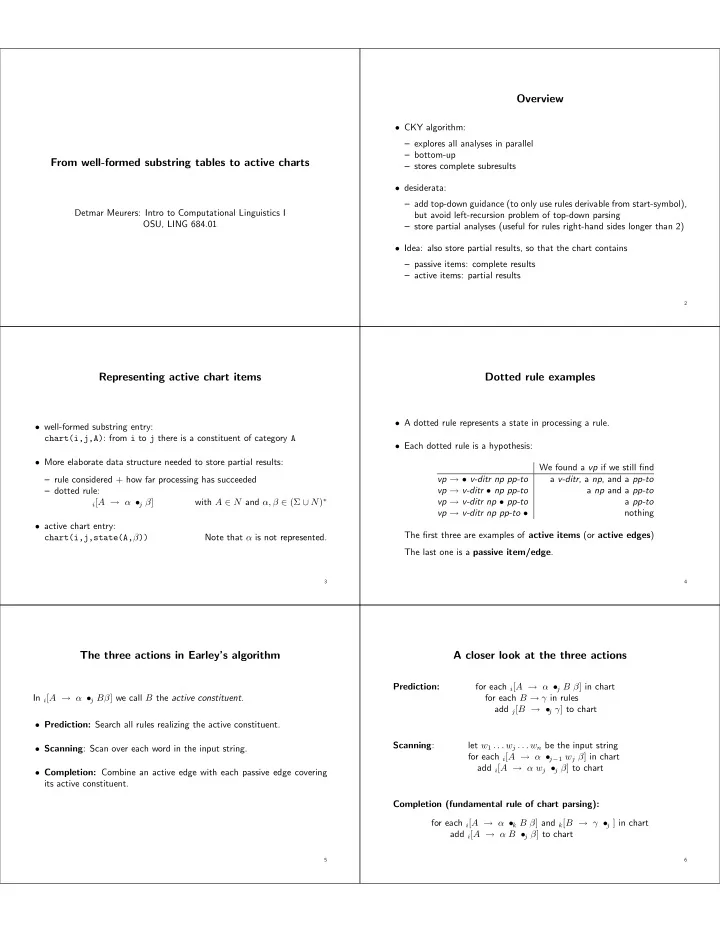
Overview • CKY algorithm: – explores all analyses in parallel – bottom-up From well-formed substring tables to active charts – stores complete subresults • desiderata: – add top-down guidance (to only use rules derivable from start-symbol), Detmar Meurers: Intro to Computational Linguistics I but avoid left-recursion problem of top-down parsing OSU, LING 684.01 – store partial analyses (useful for rules right-hand sides longer than 2) • Idea: also store partial results, so that the chart contains – passive items: complete results – active items: partial results 2 Representing active chart items Dotted rule examples • A dotted rule represents a state in processing a rule. • well-formed substring entry: chart(i,j,A) : from i to j there is a constituent of category A • Each dotted rule is a hypothesis: • More elaborate data structure needed to store partial results: We found a vp if we still find a v-ditr , a np , and a pp-to – rule considered + how far processing has succeeded vp → • v-ditr np pp-to – dotted rule: vp → v-ditr • np pp-to a np and a pp-to a pp-to i [ A → α • j β ] with A ∈ N and α, β ∈ (Σ ∪ N ) ∗ vp → v-ditr np • pp-to vp → v-ditr np pp-to • nothing • active chart entry: The first three are examples of active items (or active edges ) chart(i,j,state(A, β )) Note that α is not represented. The last one is a passive item/edge . 3 4 The three actions in Earley’s algorithm A closer look at the three actions Prediction: for each i [ A → α • j B β ] in chart In i [ A → α • j Bβ ] we call B the active constituent . for each B → γ in rules add j [ B → • j γ ] to chart • Prediction: Search all rules realizing the active constituent. Scanning : let w 1 . . . w j . . . w n be the input string • Scanning : Scan over each word in the input string. for each i [ A → α • j − 1 w j β ] in chart add i [ A → α w j • j β ] to chart • Completion: Combine an active edge with each passive edge covering its active constituent. Completion (fundamental rule of chart parsing): for each i [ A → α • k B β ] and k [ B → γ • j ] in chart add i [ A → α B • j β ] to chart 5 6
Eliminating scanning Earley’s algorithm without scanning Scanning: for each i [ A → α • j − 1 w j β ] in chart General setup: add i [ A → α w j • j β ] to chart apply prediction and completion to every item added to chart Completion: for each i [ A → α • k B β ] and k [ B → γ • j ] in chart add i [ A → α B • j β ] to chart Start: add 0 [ start → • 0 s ] to chart for each w j in w 1 . . . w n add j − 1 [ w j → • j ] to chart Observation: Scanning = completion + words as passive edges. One can thus simplify scanning to adding a passive edge for each word: for each w j in w 1 . . . w n add j − 1 [ w j → • j ] to chart Success state: 0 [ start → s • n ] 7 8 A tiny example grammar An example run start 1. 0 [ start → • 0 s ] predict from 1 2. 0 [ s → • 0 np vp ] Lexicon: predict from 2 3. 0 [ np → • 0 det n ] predict from 3 4. 0 [ det → • 0 the ] vp left → scan ”the” 5. 0 [ the → • 1 ] det the → complete 4 with 5 6. 0 [ det → the • 1 ] complete 3 with 6 7. 0 [ np → det • 1 n ] n boy → predict from 7 8. 1 [ n → • 1 boy ] n girl → predict from 7 9. 1 [ n → • 1 girl ] scan ”boy” 10. 1 [ boy → • 2 ] complete 8 with 10 11. 1 [ n → boy • 2 ] Syntactic rules: complete 7 with 11 12. 0 [ np → det n • 2 ] s np vp → complete 2 with 12 13. 0 [ s → np • 2 vp ] predict from 13 14. 2 [ vp → • 2 left ] np det n → scan ”left” 15. 2 [ left → • 3 ] complete 14 with 15 16. 2 [ vp → left • 3 ] complete 13 with 16 17. 0 [ s → np vp • 3 ] complete 1 with 17 18. 0 [ start → s • 3 ] 9 10 The Earley algorithm in Prolog (parser/earley/earley.pl) % enter_edge(+FromIndex,+ToIndex,+Contents) :- dynamic chart/3. % chart(From,To,state(Lhs,Rest_Rhs)) % a) only add if it does not yet exist: enter_edge(I,J,State) :- :- op(1200,xfx,’--->’). % operator for grammar rules chart(I,J,State), !. % recognize(+WordList,+Startsymbol): Earley recognizer toplevel % b) add to chart and make try prediction/completion recognize(String,Startsymbol) :- enter_edge(I,J,State) :- assertz(chart(I,J,State)), retractall(chart(_,_,_)), predict(I,J,State), enter_edge(0,0,state(’S’,[Startsymbol])), scan(String,0,N), complete(I,J,State). chart(0,N,state(’S’,[])). 11 12
predict(_,J,State) :- scan([],N,N). State = state(_,[B|_]), % active edge scan([W|Ws],JminOne,N) :- (B ---> Gamma), J is JminOne+1, enter_edge(J,J,state(B,Gamma)), enter_edge(JminOne,J,state(W,[])), fail scan(Ws,J,N). ; true. % ------------------------------------------------------ complete(K,J,State) :- State = state(B,[]), % passive edge chart(I,K,state(A,[B|Beta])), enter_edge(I,J,state(A,Beta)), fail ; true. 13 14 The tiny example grammar The example run in Prolog (parser/earley/earley grammar.pl) (parser parser/earley/earley trace.pl , grammar: parser/earley/earley grammar.pl ) | ?- recognize([the,boy,left]). START: 1: 0-state(S,[s])--------0 % lexicon: PRED s in 1: 2: 0-state(s,[np,vp])----0 vp ---> [left]. PRED np in 2: 3: 0-state(np,[det,n])---0 det ---> [the]. PRED det in 3: 4: 0-state(det,[the])----0 SCAN 1 (the): 5: 0-state(the,[])-------1 n ---> [boy]. COMP 4 + 5: 6: 0-state(det,[])-------1 n ---> [girl]. COMP 3 + 6: 7: 0-state(np,[n])-------1 PRED n in 7: 8: 1-state(n,[boy])------1 PRED n in 7: 9: 1-state(n,[girl])-----1 % syntactic rules: SCAN 2 (boy): 10: 1-state(boy,[])-------2 s ---> [np, vp]. COMP 8 + 10: 11: 1-state(n,[])---------2 COMP 7 + 11: 12: 0-state(np,[])--------2 np ---> [det, n]. COMP 2 + 12: 13: 0-state(s,[vp])-------2 PRED vp in 13: 14: 2-state(vp,[left])----2 SCAN 3 (left): 15: 2-state(left,[])------3 COMP 14 + 15: 16: 2-state(vp,[])--------3 COMP 13 + 16: 17: 0-state(s,[])---------3 COMP 1 + 17: 18: 0-state(S,[])---------3 SUCCESS: 18 15 16 Improving the efficiency of lexical access Code change for preterminals as passive edges (parser/earley/preterminals/earley.pl) • In the setup just described – words are stored as passive items so that scan([W|Ws],JminOne,N) :- – prediction is used for preterminal categories. The set of predicted J is JminOne+1, words for a preterminal can be huge. enter_edge(JminOne,J,state(W,[])), scan(Ws,J,N). • If each word in the grammar is introduced by a preterminal rule cat → word one can add a passive item for each preterminal category is changed to which can dominate the word instead of for the word itself. scan([W|Ws],JminOne,N) :- J is JminOne+1, • What needs to be done: ( lex(Cat,W), – syntactically distinguish syntactic rules ( ---> /2) from rules with enter_edge(JminOne,J,state(Cat,[])), preterminals on the left-hand side, i.e. lexical entries ( lex /2). fail – modify scanning to take lexical entries into account ; scan(Ws,J,N)). 17 18
The tiny example grammar in the modified format The improved example run (parser/earley/preterminals/grammar1.pl) (parser parser/earley/preterminals/earley trace.pl , grammar: parser/earley/preterminals/grammar1.pl ) | ?- recognize([the,boy,left],s). % lexicon: START: 1: 0--state(S,[s])-------0 lex(vp,left). PRED s in 1: 2: 0--state(s,[np,vp])---0 lex(det,the). PRED np in 2: 3: 0--state(np,[det,n])--0 SCAN 1 (the): 4: 0--state(det,[])------1 lex(n,boy). COMP 3 + 4: 5: 0--state(np,[n])------1 lex(n,girl). SCAN 2 (boy): 6: 1--state(n,[])--------2 COMP 5 + 6: 7: 0--state(np,[])-------2 % syntactic rules: COMP 2 + 7: 8: 0--state(s,[vp])------2 s ---> [np, vp]. SCAN 3 (left): 9: 2--state(vp,[])-------3 np ---> [det, n]. COMP 8 + 9: 10: 0--state(s,[])--------3 COMP 1 + 10: 11: 0--state(S,[])--------3 SUCCESS: 11 19 20 Towards more flexible control Earley-recognizer with explicit agenda and chart (parser/earley/agenda/earley.pl) :- op(1200,xfx,’--->’). % Operator for grammar rules The algorithms, we saw – use the Prolog database to store the chart and % Data structures: chart(From,To,Category) – Prolog backtracking on edges in chart instead of an explicit agenda. % ------------------------------------------------------ % recognize(+WordList) % top-level predicate for Earley recognizer Alternatively, one can – explicitly introduce an agenda recognize(String,Startsymbol) :- – to store and work off edges in any order one likes. StartAgenda=[chart(0,0,state(’S’,[Startsymbol]))], process_agenda(StartAgenda,[],Chart0), scan(String,0,N,Chart0,Chart), element(chart(0,N,state(’S’,[])),Chart). 21 22 % process_agenda(+Agenda,+ChartIn,-ChartOut) scan([],N,N,Chart,Chart). process_agenda([],X,X). scan([W|Ws],JminOne,N,Chart0,Chart) :- process_agenda([Edge|Agenda0],Chart0,Chart) :- J is JminOne+1, element(Edge,Chart0), !, setof(chart(JminOne,J,state(Cat,[])), process_agenda(Agenda0,Chart0,Chart). lex(Cat,W), process_agenda([Edge|Agenda0],Chart0,Chart) :- Agenda), Chart1=[Edge|Chart0], process_agenda(Agenda,Chart0,Chart1), % scan(Ws,J,N,Chart1,Chart). predict(Edge,PAgenda), append(PAgenda,Agenda0,Agenda1), % complete(Edge,Chart1,CAgenda), append(CAgenda,Agenda1,NewAgenda), process_agenda(NewAgenda,Chart1,Chart). 23 24
Recommend


More recommend
Explore More Topics
Stay informed with curated content and fresh updates.