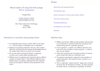
Outline Mixed models in R using the lme4 package Part 3: - PowerPoint PPT Presentation
Outline Mixed models in R using the lme4 package Part 3: Longitudinal data Longitudinal data: sleepstudy A model with random effects for intercept and slope Douglas Bates University of Wisconsin - Madison Conditional means and R Development
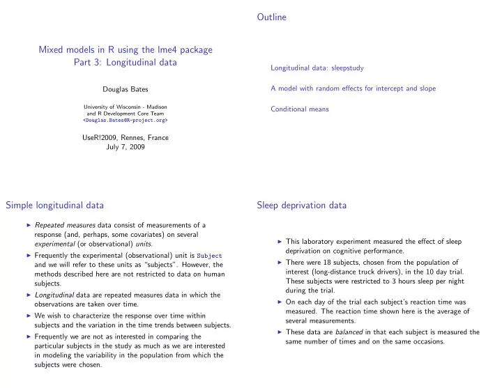
Outline Mixed models in R using the lme4 package Part 3: Longitudinal data Longitudinal data: sleepstudy A model with random effects for intercept and slope Douglas Bates University of Wisconsin - Madison Conditional means and R Development Core Team <Douglas.Bates@R-project.org> UseR!2009, Rennes, France July 7, 2009 Simple longitudinal data Sleep deprivation data ◮ Repeated measures data consist of measurements of a response (and, perhaps, some covariates) on several ◮ This laboratory experiment measured the effect of sleep experimental (or observational) units . deprivation on cognitive performance. ◮ Frequently the experimental (observational) unit is Subject ◮ There were 18 subjects, chosen from the population of and we will refer to these units as “subjects”. However, the interest (long-distance truck drivers), in the 10 day trial. methods described here are not restricted to data on human These subjects were restricted to 3 hours sleep per night subjects. during the trial. ◮ Longitudinal data are repeated measures data in which the ◮ On each day of the trial each subject’s reaction time was observations are taken over time. measured. The reaction time shown here is the average of ◮ We wish to characterize the response over time within several measurements. subjects and the variation in the time trends between subjects. ◮ These data are balanced in that each subject is measured the ◮ Frequently we are not as interested in comparing the same number of times and on the same occasions. particular subjects in the study as much as we are interested in modeling the variability in the population from which the subjects were chosen.
Reaction time versus days by subject Comments on the sleep data plot ◮ The plot is a “trellis” or “lattice” plot where the data for each subject are presented in a separate panel. The axes are consistent across panels so we may compare patterns across 0 2 4 6 8 0 2 4 6 8 0 2 4 6 8 0 2 4 6 8 351 335 332 372 333 352 331 330 337 subjects. ● ● ● 450 ● ● ● ◮ A reference line fit by simple linear regression to the panel’s 400 ● ● ● ● ● ● ● ● ● ● ● ● ● ● ● ● 350 ● ● ● ● ● ● ● ● ● ● data has been added to each panel. Average reaction time (ms) ● ● ● ● ● ● ● ● ● ● ● ● ● ● ● ● 300 ● ● ● ● ● ● ● ● ● ● ● ● ● ● ● ● ● ● ● ● ● ● ● ● ● ● ● ● ● ● ● ● ● ● ● ● ● ● 250 ● ● ● ◮ The aspect ratio of the panels has been adjusted so that a ● 200 typical reference line lies about 45 ◦ on the page. We have the 310 309 370 349 350 334 308 371 369 ● 450 ● greatest sensitivity in checking for differences in slopes when ● 400 ● ● ● ● ● ● ● the lines are near ± 45 ◦ on the page. ● ● ● ● 350 ● ● ● ● ● ● ● ● ● ● ● ● ● ● ● ● 300 ● ● ● ● ● ● ● ● ● ● ● ● ● ● ● ● ● ● ● ● ● ◮ The panels have been ordered not by subject number (which ● ● ● ● ● ● ● ● ● ● 250 ● ● ● ● ● ● ● ● ● ● ● ● ● ● ● ● ● ● ● ● ● ● ● ● ● ● ● 200 ● ● is essentially a random order) but according to increasing 0 2 4 6 8 0 2 4 6 8 0 2 4 6 8 0 2 4 6 8 0 2 4 6 8 intercept for the simple linear regression. If the slopes and the Days of sleep deprivation intercepts are highly correlated we should see a pattern across the panels in the slopes. Assessing the linear fits 95% conf int on within-subject intercept and slope ◮ In most cases a simple linear regression provides an adequate fit to the within-subject data. (Intercept) Days ◮ Patterns for some subjects (e.g. 350, 352 and 371) deviate 337 | | | | 330 | | | | 331 | | | | from linearity but the deviations are neither widespread nor 352 | | | | 333 | | | | consistent in form. 372 | | | | 332 | | | | 335 | | | | ◮ There is considerable variation in the intercept (estimated 351 | | | | 369 | | | | reaction time without sleep deprivation) across subjects – 200 371 | | | | 308 | | | | 334 | | | | ms. up to 300 ms. – and in the slope (increase in reaction 350 | | | | 349 | | | | time per day of sleep deprivation) – 0 ms./day up to 20 370 | | | | 309 | | | | 310 | | | | ms./day. 180 200 220 240 260 280 −10 0 10 20 ◮ We can examine this variation further by plotting confidence intervals for these intercepts and slopes. Because we use a pooled variance estimate and have balanced data, the These intervals reinforce our earlier impressions of considerable intervals have identical widths. variability between subjects in both intercept and slope but little evidence of a relationship between intercept and slope. ◮ We again order the subjects by increasing intercept so we can check for relationships between slopes and intercepts.
A preliminary mixed-effects model Fitting the model > (fm1 <- lmer(Reaction ~ Days + (Days | Subject), ◮ We begin with a linear mixed model in which the fixed effects + sleepstudy)) [ β 1 , β 2 ] ′ are the representative intercept and slope for the Linear mixed model fit by REML population and the random effects Formula: Reaction ~ Days + (Days | Subject) b i = [ b i 1 , b i 2 ] ′ , i = 1 , . . . , 18 are the deviations in intercept and Data: sleepstudy AIC BIC logLik deviance REMLdev slope associated with subject i . 1756 1775 -871.8 1752 1744 ◮ The random effects vector, b , consists of the 18 intercept Random effects: effects followed by the 18 slope effects. Groups Name Variance Std.Dev. Corr Subject (Intercept) 612.092 24.7405 Days 35.072 5.9221 0.066 Residual 654.941 25.5918 Number of obs: 180, groups: Subject, 18 Fixed effects: 10 Estimate Std. Error t value 20 (Intercept) 251.405 6.825 36.84 Days 10.467 1.546 6.77 30 50 100 150 Correlation of Fixed Effects: (Intr) Days -0.138 Terms and matrices A model with uncorrelated random effects ◮ The data plots gave little indication of a systematic relationship between a subject’s random effect for slope and his/her random effect for the intercept. Also, the estimated correlation is quite small. ◮ The term Days in the formula generates a model matrix X ◮ We should consider a model with uncorrelated random effects. with two columns, the intercept column and the numeric Days To express this we use two random-effects terms with the column. (The intercept is included unless suppressed.) same grouping factor and different left-hand sides. In the ◮ The term (Days|Subject) generates a vector-valued random formula for an lmer model, distinct random effects terms are effect (intercept and slope) for each of the 18 levels of the modeled as being independent. Thus we specify the model Subject factor. with two distinct random effects terms, each of which has Subject as the grouping factor. The model matrix for one term is intercept only ( 1 ) and for the other term is the column for Days only, which can be written 0+Days . (The expression Days generates a column for Days and an intercept. To suppress the intercept we add 0+ to the expression; -1 also works.)
Recommend
More recommend
Explore More Topics
Stay informed with curated content and fresh updates.
