Other Related Problems Applications Classification Instance - PowerPoint PPT Presentation
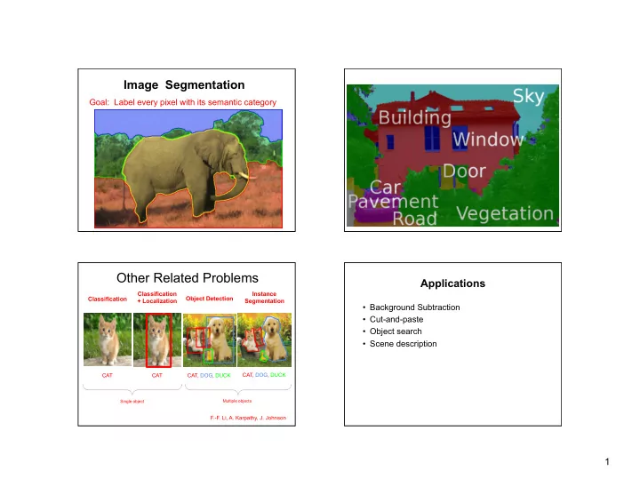
Image Segmentation Goal: Label every pixel with its semantic category * Other Related Problems Applications Classification Instance Classification Object Detection + Localization Segmentation Background Subtraction Cut-and-paste
Image Segmentation Goal: Label every pixel with its semantic category * Other Related Problems Applications Classification Instance Classification Object Detection + Localization Segmentation • Background Subtraction • Cut-and-paste • Object search • Scene description CAT CAT CAT, DOG, DUCK CAT, DOG, DUCK Single object Multiple objects Lecture 8 - F.-F. Li, A. Karpathy, J. Johnson 1
Some Hard Examples From Images to Objects • What Defines an Object? • How to Find Objects? – Find boundaries between objects – Find “cohesive” regions 2
What is Segmentation? Some Criteria for Segmentation • Clustering image elements that “ belong together ” – Partitioning • Pixels within a region should have similar • Divide into regions with coherent internal properties appearance, i.e., the statistics of their pixel – Grouping intensities, colors, textures, etc. should fit some • Identify sets of coherent tokens in image model. Region should be compact. • Tokens: Whatever we need to group – Pixels • The boundaries between regions should – “Superpixels” (regions with small range of color or – Have discontinuities in color or texture or … texture) – Smooth or piecewise smooth or … – Features (corners, lines, etc.) Human Vision: Figure-Ground Segmentation Approaches to Image Segmentation • Segmentation by Humans • Manual Segmentation with Games • Automatic Segmentation Methods • Interactive Segmentation Methods 3
For the human visual system, Gestalt psychology identifies several properties that result in grouping/ segmentation: For the human visual system, Gestalt psychology Groupings by Invisible Completions identifies several properties that result in grouping/ segmentation: * Images from Steve Lehar ’ s Gestalt papers: http://cns-alumni.bu.edu/pub/slehar/Lehar.html 4
Image Segmentation by Humans LabelMe Goals • The goal of LabelMe is to provide an online annotation tool to build a large database of annotated (= roughly segmented and labeled ) images by collecting contributions from many people • Large set of scenes (indoor, outdoor) and many object classes in context • Collect the large, high quality database of annotated images • Images come from multiple sources, taken at many cities/countries (to help avoid overfitting) • Allow researchers immediate access to the latest LabelMe version of the database • LabelMe Matlab toolbox http://labelme.csail.mit.edu/ Bryan Russell LabelMe Screen Shot 5
Segmentation as Clustering boat • Cluster together (pixels, tokens, etc.) that belong together • Agglomerative clustering – attach to cluster it is closest to – repeat • Divisive clustering – split cluster along best boundary – repeat Histogram-Based Segmentation: Histogram-Based Segmentation: A Simple Agglomerative Clustering Method A Simple Agglomerative Clustering Method • Goal • Goal – Segment the image into K regions – Segment the image into K regions – Solve this by reducing the number of colors to K – Solve this by reducing the number of colors to K and mapping each pixel to the closest color and mapping each pixel to the closest color 6
K-Means Clustering K-Means Clustering • The dataset. Input k =5 • K-means clustering algorithm 1. Randomly initialize the cluster centers, c 1 , ..., c K 2. Given cluster centers, determine points in each cluster • For each point p , find the closest c i . Put p in cluster i 3. Given points in each cluster, solve for c i • Set c i to be the mean of points in cluster i 4. If c i have changed, go to Step 2 • Properties – Will always converge to some solution – Can be a “ local minimum ” • does not always find the global minimum of objective function: K-Means Clustering K-Means Clustering Each point finds Randomly pick 5 which cluster center posi?ons as ini?al it is closest to; the cluster centers (not point belongs to that necessarily data cluster points) 7
K-Means Clustering K-Means Clustering Each cluster Each cluster computes its new computes its new centroid, based on centroid based on which points belong which points belong to it to it Repeat un?l convergence (i.e., no cluster center moves) Image Segmentation using K-Means Example • Select a value of K • Select a feature vector for every pixel (color, texture, position, etc.) • Define a similarity measure between feature vectors (e.g., Euclidean Distance) • Apply K-Means algorithm • Apply Connected Components algorithm • Merge any components of size less than some threshold to an adjacent component that is most Image Clusters on intensity Clusters on color similar to it 8
Mean Shift Algorithm D. Comaniciu and P. Meer Mean Shift Algorithm Intuitive Description Region of Mean Shift Algorithm interest 1. Choose a search window size Center of 2. Choose the initial location of the search window mass 3. Compute the mean location (centroid of the data) in the search window 4. Center the search window at the mean location computed in Step 3 5. Repeat Steps 3 and 4 until convergence The mean shift algorithm seeks the mode , i.e., point of highest density of a data distribution: Mean Shift vector Objective : Find the densest region Distribution of identical billiard balls 9
Intuitive Description Intuitive Description Region of Region of interest interest Center of Center of mass mass Mean Shift Mean Shift vector vector Objective : Find the densest region Objective : Find the densest region Distribution of identical billiard balls Distribution of identical billiard balls Intuitive Description Intuitive Description Region of Region of interest interest Center of Center of mass mass Mean Shift Mean Shift vector vector Objective : Find the densest region Objective : Find the densest region Distribution of identical billiard balls Distribution of identical billiard balls 10
Intuitive Description Intuitive Description Region of Region of interest interest Center of Center of mass mass Mean Shift vector Objective : Find the densest region Objective : Find the densest region Distribution of identical billiard balls Distribution of identical billiard balls Results Results 11
Graph-based Clustering: Results Images as Graphs q affinity pq affinity p • Fully-connected graph – node for every pixel – link between pairs of pixels, p , q – cost affinity pq for each link • affinity pq measures similarity – similarity is inversely proportional to difference in color, texture, etc. The Image as a Graph Affinity (Similarity) Measures • Intensity Node: pixel 2 2 − − σ = I ( ) x I ( ) y /2 aff( , ) x y e I Edge: affinity between two • Distance pixels 2 2 − − σ 2 x y / = aff( x , y ) e d • Color • Texture • Motion 12
Problem Formulation • Let A, B partition G. Therefore, A ∪ B = V , and A ∩ B = ∅ • Given an undirected graph G = ( V , E ), where V is a set of nodes, one for each data element (e.g., • The dissimilarity between A and B is defined as pixel), and E is a set of edges with weights ∑ cut (A,B) = affinity representing the affinity between connected ij i A j B ∈ , ∈ nodes = total weight of edges removed • Find the image partition that maximizes the • The optimal bi-partition (i.e., segment image “ similarity ” within each region and minimizes into 2 regions) of G is the one that minimizes cut the “ dissimiliarity ” between regions • Finding the optimal partition is NP-complete Image Segmentation & Minimum Cut Pixel Neighborhood w Image Pixels Similarity Measure Minimum Cut * From Khurram Hassan-Shafique CAP5415 Computer Vision 2003 13
• So, instead define the normalized similarity, called the normalized-cut (A, B), as cut ( A , B ) cut ( B , A ) = + ncut ( A , B ) assoc ( A , V ) assoc ( B , V ) ∑ where assoc ( A , V ) = affinity ik ∈ ∈ i A k V , = total connection weight from nodes in A to all nodes in G • Ncut removes the bias based on region size • New goal: Find bi-partition that minimizes ncut (A, B) • Can be found in polynomial time in number of pixels Results Synthetic Image Results 14
K-Means vs. Mean Shift vs. Results Normalized Cut Some Weaknesses of Normalized Cut Interactive Image Segmentation • Boundary-based methods • Very large storage requirement – Intelligent scissors • Bias towards partitioning into equal segments • Uses local edge information • Often over-segments – Snakes / Active contours • Has problems with textured backgrounds • Uses local edge information and contour smoothness • Graph-cut methods – GrabCut • Uses boundary and region terms * Slide from Khurram Hassan-Shafique CAP5415 Computer Vision 2003 15
Recommend
More recommend
Explore More Topics
Stay informed with curated content and fresh updates.
