Other Continuous Distributions Weibull Distribution Suppose that X - PowerPoint PPT Presentation

ST 380 Probability and Statistics for the Physical Sciences Other Continuous Distributions Weibull Distribution Suppose that X has the standard exponential distribution, so F X ( x ) = P ( X ≤ x ) = 1 − e − x , x ≥ 0 . Now suppose that W = β X 1 /α for some α > 0 and β > 0. Then F W ( w ) = 0 for w < 0, and for w ≥ 0 � α � � � w F W ( w ) = P ( W ≤ w ) = P ( β X 1 /α ≤ w ) = P X ≤ β = 1 − e − ( w /β ) α . W has the Weibull distribution with parameters α and β . 1 / 10 Continuous Random Variables Other Distributions

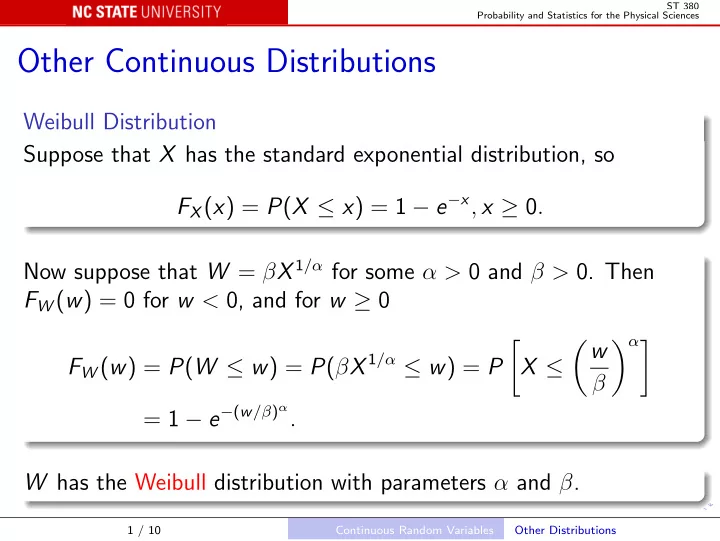
ST 380 Probability and Statistics for the Physical Sciences The pdf of the Weibull distribution is found by differentiating F W ( w ). Like the gamma family, the Weibull family includes the exponential distribution as a special case, here when α = 1. Weibull distributions have been used as models for failure times in survival analysis and reliability theory and for various physical measurements. 2 / 10 Continuous Random Variables Other Distributions

ST 380 Probability and Statistics for the Physical Sciences Lognormal Distribution Suppose that X ∼ N ( µ, σ 2 ), so that � x − µ � P ( X ≤ x ) = Φ . σ Now suppose that Y = e X . Then F Y ( y ) = 0 for y ≤ 0, and for y > 0 � log y − µ � F Y ( y ) = P ( Y ≤ y ) = P ( e X ≤ y ) = P ( X ≤ log y ) = Φ . σ Y has the lognormal distribution with parameters µ and σ . 3 / 10 Continuous Random Variables Other Distributions

ST 380 Probability and Statistics for the Physical Sciences The pdf of the lognormal distribution is found by differentiating F Y ( y ). The pdfs in the lognormal family are less varied in shape than those of the gamma and Weibull families, but have been found useful as models for particle size distributions and air pollution levels. They also play a prominent role in the Black-Scholes theory of the prices of financial options such as puts and calls. 4 / 10 Continuous Random Variables Other Distributions

ST 380 Probability and Statistics for the Physical Sciences Beta Distribution The gamma, Weibull, and lognormal families are models for non-negative and unbounded continuous random variables. The beta family is a model for a bounded continuous random variable. In the simplest case, the range of X is (0 , 1), and for parameters α > 0 and β > 0, the pdf is � Γ( α + β ) Γ( α )Γ( β ) x α − 1 (1 − x ) β − 1 0 < x < 1 f ( x ; α, β ) = 0 otherwise. If the variable should have a more general range ( A , B ), use the variable Y = A + ( B − A ) X . 5 / 10 Continuous Random Variables Other Distributions

ST 380 Probability and Statistics for the Physical Sciences The beta family includes the uniform distribution as the special case α = β = 1. Wigner’s semi-circle density is another special case, with α = β = 1 . 5 and A = − B : √ � B 2 − x 2 2 | x | < B π B 2 f ( x ; 1 . 5 , 1 . 5 , − B , B ) = 0 | x | ≥ B . Applications of the beta family include: the distribution of grades on an exam ( A = 0 , B = 100); amounts recovered in a bankruptcy (if in cents per dollar, A = 0 , B = 100; if as a fraction, A = 0 , B = 1). 6 / 10 Continuous Random Variables Other Distributions

ST 380 Probability and Statistics for the Physical Sciences Probability Plots Many statistical procedures depend on assumptions about the nature of the data being analyzed, such as that they are normally distributed. So we need ways to explore whether such assumptions are correct. The quantile-quantile plot (or q-q plot) is a graphical tool for doing that. 7 / 10 Continuous Random Variables Probability Plots

ST 380 Probability and Statistics for the Physical Sciences The basic idea is to plot the quantiles (percentiles) of the distribution of one random variable against those of another. If they are all the same, the graph is the identity line y = x , and the distributions are identical. If the graph is some other straight line, the distributions are in the same location-scale family. Suppose for example that X ∼ N (0 , 1) and Y ∼ N ( µ, σ 2 ). We have seen that η Y ( p ) = µ + ση X ( p ) , so the graph of η Y ( p ) against η X ( p ) is the straight line y = µ + σ x . 8 / 10 Continuous Random Variables Probability Plots

ST 380 Probability and Statistics for the Physical Sciences In practice, we may know (or hypothesize) the distribution of X , for example as the standard normal distribution, but have only a sample of values from the distribution of Y . So we estimate the quantiles of the distribution of Y , and plot the estimates of those quantiles against those of X . For instance, the median of the sample values is an estimate of the median of the distribution of Y , the sample quartiles estimate the quartiles of the distribution of Y , and so on. 9 / 10 Continuous Random Variables Probability Plots

ST 380 Probability and Statistics for the Physical Sciences More generally, if the ordered sample values are � � i − 1 / 2 y (1) ≤ y (2) ≤ · · · ≤ y ( n ) , then y ( i ) estimates η Y . n A q-q plot is a graph of � i − 1 / 2 � � i − 1 / 2 � η Y ˆ = y ( i ) against η X , i = 1 , 2 , . . . , n . n n The R function qqnorm() actually plots � � i − a y ( i ) against η X , n + 1 − 2 a where a = 3 / 8 for n ≤ 10 and a = 1 / 2 otherwise. 10 / 10 Continuous Random Variables Probability Plots