Order Reduction of Large Scale DAE Models J.D. Hedengren and T. F. - PowerPoint PPT Presentation
Order Reduction of Large Scale DAE Models J.D. Hedengren and T. F. Edgar Department of Chemical Engineering The University of Texas at Austin 1 Outline Motivation Two Step Process for DAE Model Reduction 1. Reduction of
Order Reduction of Large Scale DAE Models J.D. Hedengren and T. F. Edgar Department of Chemical Engineering The University of Texas at Austin 1
Outline • Motivation • Two Step Process for DAE Model Reduction 1. Reduction of differential equations 2. Reduction of algebraic equations with ISAT • Examples 2
DAE model size • Small (1-100 variables) – Single process units (e.g., reactor models) – Real-time NMPC calculations are feasible • Medium (100-10,000 variables) – Multiple process units – Multicomponent modeling, reaction networks – Real-time NMPC applications very difficult • Large (10,000+ variables) – Plant wide dynamic models – Currently optimized at this level only with steady state models (RTO) 3
Motivation • Plantwide NMPC control (Large scale DAE systems) • Storage and retrieval of optimal control trajectories (small and medium scale) • Reveal underlying structure of the model – Determine dynamic degrees of freedom – Find source of DAE initialization / convergence problems • Automate model reduction 4
Adaptive DAE Model Reduction 1. Reduction of differential equations 2. Reduction of algebraic equations 5
ODE Model Reduction • Optimally reduce the number of model variables • Linear combination of states that retain the most important dynamics • Methods – Proper Orthogonal Decomposition (POD) – Balanced Covariance Matrices (BCM) 6
Predicting DDOF • Can model reduction be made adaptive? • Possible error control strategies: – Singular values (poor predictor) – Solve non-reduced model at check points (inefficient) – Equation residuals (new approach) 7
Model Reduction Error • Variable error constraint x ( ) t − x t ( ) ≤ ε ROM tol • Controlling variable error – ↓ model order, ↑ variable error – ↑ model order, ↓ variable error • DOF – Total degrees of freedom (DOF) = model order – Dynamic degrees of freedom (DDOF) = reduced model order that satisfies the variable error constraint 8
Predicting DDOF • Linearized system ɺ x ( t ) = Ax ( t ) + Bu ( t ) • Galerkin projection ~ T x ( t ) = P x ( t ) + r ( t ) ~ T ɺ ɺ ɺ x ( t ) = P x ( t ) + r ( t ) • Substitute ~ ( ~ ) T T ɺ ɺ P x ( t ) = A P x ( t ) + Ar ( t ) − r ( t ) + Bu ( t ) • Predictor ( r(t) = variable error, R(t) = equation residual ) ɺ R ( t ) = Ar ( t ) − r ( t ) ≅ Ar ( t ) − 1 r ( t ) ≅ A R ( t ) Variable error predictor (linearized) 9
Adaptive ODE Model Reduction • Variable error constraint − 1 x ( ) t − x t ( ) = r t ( ) ≅ A R t ( ) ≤ ε ROM tol • Open equation format f ɺ ( x ( t ), x ( t )) = 0 Solution obtained by finding roots ~ ~ T T ɺ f ( P x ( t ), P x ( t )) = R ( t ) Solution obtained by minimizing residuals • Controlling variable error (iterative approach) − 1 – When , ↓ model order A R ( t ) ≤ ε tol − 1 A R ( t ) > ε – When , ↑ model order tol • Variable error predictor can also be used to improve reduced model accuracy 10
Example: Adaptive ODE Reduction • 1-D unsteady heat conduction T 1 T 2 ∂ T ∂ ∂ T ρ c = k ∂ t ∂ x ∂ x • Discretized the PDE to give a set of 20 ODEs • Simulation: – Aluminum slab with thickness 1 m – Initially at 25 ºC – At t = 0 the left boundary is changed to 100 ºC – Tolerance set ε tol = 1 ºC 11
Example Results • After 100 minutes the temperature profile approaches steady state 20 states 400 3 states 2 states 380 1 state ) K ( e 360 r u t a r e p 340 m e T 320 300 0 0.2 0.4 0.6 0.8 1 Distance (m) • Variable error predictor indicates that at least 3 states are required to meet error tolerance of 1 ºC 12
Example Results • Variable error predictor can also be used to improve the reduced model accuracy (1 state required with correction) 380 20 states 370 3 states 2 states 360 1 state ) C º ( 350 e r u t 340 a r e p 330 m e T 320 310 300 0 0.2 0.4 0.6 0.8 1 Distance (m) • Excellent prediction because the model is nearly linear and approaching steady state 13
Adaptive DAE Model Reduction 1. Reduction of differential equations (model reduction) 2. Reduction of algebraic equations with ISAT 14
Partitioning and Precedence Ordering • DAE model f ODE ɺ ( x , x , y , t ) = 0 f DAE ɺ ( z , z , t ) = 0 f ( x , y , t ) = 0 AE x = ODE state; y = algebraic state • Sparsity matrix 1 if y or x ɺ appears in f j j DAE i J = ij 0 otherwise • Pairing equations and variables – Obtain a maximum transversal (largest diagonal via rearrangement) – Zero-free diagonal means that each variable is uniquely paired with an equation 15
Partitioning and Precedence Ordering • Lower triangular block form – Each successive block of variables and equations can be solved independently – Inverting the sparsity matrix shows global variable dependencies – Binary distillation example (230 x 230 system): Original sparsity Lower triangular block form ɺ X 0 X 0 0 X 0 0 0 0 x X X X 0 0 0 0 0 0 0 T A sat ɺ 0 X 0 0 0 X X X 0 0 h X X X 0 0 0 0 0 0 0 P A sat 0 0 X 0 0 0 0 0 X 0 y X X X 0 0 0 0 0 0 0 P A B 0 0 0 X 0 0 X X 0 0 x X X X X 0 0 0 0 0 0 h L L X X T 0 0 0 0 0 0 0 0 X X X 0 X 0 0 0 0 0 y A ɺ ɺ 0 0 0 X 0 X 0 0 0 0 n or n X X X 0 X X 0 0 0 0 h V L V 0 0 X 0 X 0 X 0 0 0 h X X X X X X X 0 0 0 x V L 0 0 0 0 X 0 0 X 0 0 h ɺ ɺ X X X X X X X X 0 0 n or n L V L sat 0 0 0 0 X 0 0 0 X 0 P ɺ X X X X X X X X X 0 x A A sat ɺ 0 0 0 0 X 0 0 0 0 X P X X X X X X X X 0 X h B 16
Scalability to Large Systems • n – number of algebraic equations • τ – number of non-zeros in the sparsity matrix • The maximum transversal algorithm has a worst case bound of O(n τ ) although typical examples are more like O(n) + O( τ ) (Duff, 1981) • The lower triangular block algorithm also exhibits excellent scaling for large problems with an upper bound of O(n) + O( τ ) (Duff and Reid, 1978) • Similar to approaches for solving process design equations (1970s) 17
Reduction of Algebraic Equations • Explicit transformation of algebraic equations – Transform model equations into an explicit form • Apply Tarjan’s algorithm for precedence ordering – Model equations can be proprietary (not available to user, e.g. commercial simulator) – Neural networks • Extrapolation problems • No reliable error control strategy – In situ adaptive tabulation (ISAT) • Dynamic database with error control • Replacement for neural nets? 18
Example: Flowsheet Modeling and Model Reduction • Multicomponent, multiphase object-oriented simulator • FORTRAN 90 routines for fast execution • DIPPR database with properties for >1700 compounds • DASPK 3.0 for numerical integration and sensitivity analysis • Current models are a compressor, splitter, mixer, vessel, heat exchanger, and flash column 19
Example: Flowsheet Model • Blending and separation – Feed streams: butane, pentane, hexane, heptane, and octane • DAE model – 12 differential equations – 217 algebraic equations Feed 1 Feed 2 Product 1 Product 2 Mixer Split Holding F valve Tank l Heat a Exchanger s h Product 3 20
Example: Reduced Flowsheet Model Results • Algebraic equation decomposition – 202 successively independent sets of variables and equations – One implicit set: 16 equations (flash column) – Model reduced from 229 to 28 states – 12 ODEs / 16 AEs Feed 1 Feed 2 Product 1 Product 2 Mixer Split Holding F valve Tank l Heat a Exchanger s h Product 3 21
Example: ISAT vs. Neural Nets • Nonlinear function test case (2 independent variables) – 1 st eigenfunction of an L-shaped membrane – 2 nd and 3 rd eigenfunctions also appear on Mathworks’ publications – Linear and nonlinear regions – Points that are not continuously differentiable – ISAT also handles function discontinuities, although that capability is not demonstrated here 22
ISAT • Principal tuning parameter ( ε tol ) – Set to ε tol = 0.5 (extremely coarse) – Intuitive adjustable parameter – in this case little accuracy is required – ISAT created 12 linear regions ( x 1 , x 2 , f ) 23
Recommend
More recommend
Explore More Topics
Stay informed with curated content and fresh updates.


