Order Recursion Introduction Introduction Rc = d Order versus Time - PowerPoint PPT Presentation
Order Recursion Introduction Introduction Rc = d Order versus Time Updates There are many ways to solve the normal equations Matrix Inversion by Partitioning Lemma Solutions are mathematically equivalent Levinson Algorithm
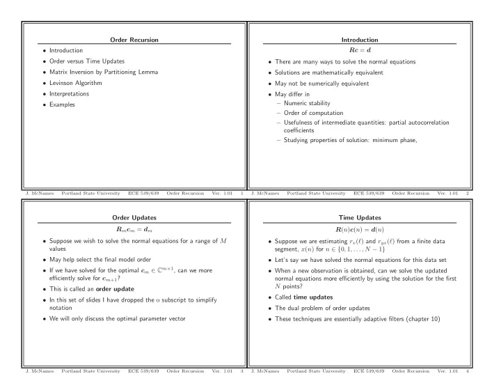
Order Recursion Introduction • Introduction Rc = d • Order versus Time Updates • There are many ways to solve the normal equations • Matrix Inversion by Partitioning Lemma • Solutions are mathematically equivalent • Levinson Algorithm • May not be numerically equivalent • Interpretations • May differ in – Numeric stability • Examples – Order of computation – Usefulness of intermediate quantities: partial autocorrelation coefficients – Studying properties of solution: minimum phase, J. McNames Portland State University ECE 539/639 Order Recursion Ver. 1.01 1 J. McNames Portland State University ECE 539/639 Order Recursion Ver. 1.01 2 Order Updates Time Updates R m c m = d m R ( n ) c ( n ) = d ( n ) • Suppose we wish to solve the normal equations for a range of M • Suppose we are estimating r x ( ℓ ) and r yx ( ℓ ) from a finite data values segment, x ( n ) for n ∈ { 0 , 1 , . . . , N − 1 } • May help select the final model order • Let’s say we have solved the normal equations for this data set • If we have solved for the optimal c m ∈ C m × 1 , can we more • When a new observation is obtained, can we solve the updated efficiently solve for c m +1 ? normal equations more efficiently by using the solution for the first N points? • This is called an order update • Called time updates • In this set of slides I have dropped the o subscript to simplify notation • The dual problem of order updates • We will only discuss the optimal parameter vector • These techniques are essentially adaptive filters (chapter 10) J. McNames Portland State University ECE 539/639 Order Recursion Ver. 1.01 3 J. McNames Portland State University ECE 539/639 Order Recursion Ver. 1.01 4
Scope of Order Updates Stationary Case R m c m = d m Rc = d • The text covers all of the cases we have discussed • When the process is stationary, R is Toeplitz – Any linear estimation problem • This permits more efficient algorithms to be used – Optimum FIR filters • In general the inversion of an M × M matrix requires O ( M 3 ) – Optimum FIR filters for stationary processes operations • While the solutions are insightful for the first two cases, they are • When R is Toeplitz we can no more efficient computationally – Invert the matrix in O ( M 2 ) operations – Perform an LDL H decomposition in O ( M 2 ) operations • We will only discuss the last case • See Section 7.7 for details • We will consider both the stationary FIR filter and nonstationary linear combiner cases J. McNames Portland State University ECE 539/639 Order Recursion Ver. 1.01 5 J. McNames Portland State University ECE 539/639 Order Recursion Ver. 1.01 6 Linear Combiner: Notation Inversion of Partitioned Hermitian Matrices In this set of notes and m subscript is used to indicate the size of m and we wish to compute R − 1 • Suppose we know R − 1 m +1 efficiently matrices and vectors so that we can solve the normal equations R m +1 c m +1 = d m +1 �� � � �� � R m � x m r b m • The inverse of a Hermitian matrix is also Hermitian x H R m +1 = E = x ∗ m +1 r H m x m +1 ρ b m b m • We are not assuming R m is Toeplitz yet �� x m � d m � � � d m +1 = E [ x m +1 y ∗ ] = E y ∗ = x m +1 d m +1 � Q m � q m Q m +1 � R − 1 = Q H m +1 = q H m +1 where q m m | x m +1 | 2 � r b m � E � � ρ b m � E � x m x ∗ � R m � � Q m � � I m � m +1 r b m q m 0 m R m +1 Q m +1 = = r H q H 0 H ρ b m q m 1 b m m m R m Q m + r b m q H r H b m Q m + ρ b m q H m = 0 H m = I m m r H R m q m + r b m q m = 0 m b m q m + ρ b m q m = 1 J. McNames Portland State University ECE 539/639 Order Recursion Ver. 1.01 7 J. McNames Portland State University ECE 539/639 Order Recursion Ver. 1.01 8
Inversion of Partitioned Hermitian Matrices Continued Inversion of Partitioned Hermitian Matrices Continued R m Q m + r b m q H r H b m Q m + ρ b m q H m = 0 H 1 m = I m m q m = b m R − 1 ρ b m − r H m r b m r H R m q m + r b m q m = 0 m b m q m + ρ b m q m = 1 − R − 1 m r b m q m = We only have three unknowns, so only three of these equations are b m R − 1 ρ b m − r H m r b m needed to obtain the solutions. m + R − 1 m r b m ( − R − 1 m r b m ) H Q m = R − 1 q m = − R − 1 m r b m q m b m R − 1 ρ b m − r H m r b m 1 q m = Now if we define b m R − 1 ρ b m − r H m r b m b m � − R − 1 α b m � ρ b m − r H b m R − 1 m r b m = ρ b m + r H m r b m b m b m − R − 1 m r b m q m = b m R − 1 ρ b m − r H m r b m The we can simplify the expressions for the components of Q m +1 as m + R − 1 m r b m ( − R − 1 m r b m ) H Q m = R − 1 m − R − 1 m r b m q H m = R − 1 m + b m b H 1 q m = b m Q m = R − 1 b m R − 1 m ρ b m − r H q m = m r b m α b m α b m α b m J. McNames Portland State University ECE 539/639 Order Recursion Ver. 1.01 9 J. McNames Portland State University ECE 539/639 Order Recursion Ver. 1.01 10 Matrix Inversion by Partitioning Lemma Matrix Inversion Counterpart Following similar steps, we can show m + b m b H 1 q m = b m Q m = R − 1 m q m = � 0 � − 1 r H 0 H α b m α b m α b m � � 1 � � � ρ f m 1 R − 1 m +1 � f m m a H � = + 1 R − 1 m r f m R f m 0 m a m α f m We can then express R − 1 m +1 as f m where ⎡ ⎤ � m + b m b H � R − 1 b m � Q m � q m m R − 1 α b m α b m a m � − R − 1 α f m � ρ f m + r H f m R − 1 m +1 = = f m r f m f m r f m q H ⎣ ⎦ b H q m 1 m m α b m α b m � R − 1 � 1 � b m � � 0 m m b H � = + 1 0 H m 0 1 α b m m • This is a rank-one modification • Called the matrix inversion by partitioning lemma J. McNames Portland State University ECE 539/639 Order Recursion Ver. 1.01 11 J. McNames Portland State University ECE 539/639 Order Recursion Ver. 1.01 12
Interpretations Hermitian Inversion Summary b m = − R − 1 m r b m � T x m +1 = x m +1 + b H � e b m = x m +1 − ˆ x 1 x 2 . . . x m m α b m = ρ b m + r H b m b m � T = x 1 + a H e f m = x 1 − ˆ � x 2 x 1 x 3 . . . x m +1 m � R − 1 � 1 � � � 0 m b m R − 1 m b H � m +1 = + 1 and 0 H 0 1 m α b m m P b m = ρ b m − r H b m R − 1 • We have shown that we can obtain the inverse of R m +1 from the m r b m = α b m inverse of R m with a rank one update P f m = ρ f m − r H f m R − 1 f m r f m = α f m • Requires the R − 1 m and α b m be invertible • The vector b m is the MMSE estimator of the last element of • Applies to any Hermitian matrix x m +1 from the first m elements • The update requires O ( m 2 ) operations • Similarly, a m is the MMSE estimator of the first element of x m +1 • Is more efficient than solving the normal equations repeatedly for from the last m elements every m of interest • If x m +1 = � x ( n ) x ( n − 1) x ( n − m ) � . . . , then these are the • Is not more efficient if only c M is of interest forward (FLP) and backward (BLP) linear predictors • But how is c m +1 is related to c m ? J. McNames Portland State University ECE 539/639 Order Recursion Ver. 1.01 13 J. McNames Portland State University ECE 539/639 Order Recursion Ver. 1.01 14 Order Updates of Parameter Vectors Order Updates of Parameter Vectors Discussion c m +1 = R − 1 b m = − R − 1 α b m = ρ b m + r H m +1 d m +1 m r b m b m b m � R − 1 � � � 1 � � � � � � k c m � β c m d m b m d m 0 m β c m � b H m b H m d m + d m +1 = + 1 0 H m 0 1 d m +1 d m +1 α b m α b m m � b H � R − 1 � c m � � b m � � 1 � b m � � R − 1 0 m � � � m d m + d m +1 m d m b m R − 1 b H m � c m +1 = + k c m m +1 = + 1 = + 0 H m 0 1 0 1 α b m 0 1 α b m m � � � � c m b m • The update equation for c m +1 is called a Levinson recursion = + k c m 0 1 • If we know b m , we can determine c m +1 where • However, solving for b m requires a matrix-vector product which requires O ( m 2 ) operations for the update to c m +1 k c m � β c m β c m � b H m d m + d m +1 α b m • Contrary to the text, this approach is more efficient than solving for c m +1 = R − 1 m +1 d m +1 directly, which would require O ( m 3 ) Here the c subscript is presumably an indicator that these coefficients operations are for updating the parameter vector c • We can do even better if R m +1 is Toeplitz J. McNames Portland State University ECE 539/639 Order Recursion Ver. 1.01 15 J. McNames Portland State University ECE 539/639 Order Recursion Ver. 1.01 16
Recommend
More recommend
Explore More Topics
Stay informed with curated content and fresh updates.
