Optimizing monitoring networks for Optimizing monitoring networks - PowerPoint PPT Presentation
Optimizing monitoring networks for Optimizing monitoring networks for Optimizing monitoring networks for Optimizing monitoring networks for the detection of contaminant dispersion the detection of contaminant dispersion the detection of
Optimizing monitoring networks for Optimizing monitoring networks for Optimizing monitoring networks for Optimizing monitoring networks for the detection of contaminant dispersion the detection of contaminant dispersion the detection of contaminant dispersion the detection of contaminant dispersion A case study using the dispersion of a radioactive plume (model) in the first phase after a nuclear accident S.J. Melles, J. Beekhuizen, S. de Bruin, G.B.M. Heuvelink, A. van Dijk and C.J.W. Twenhöfel
Monitoring gamma-dose rate measurements � Chernobyl (1986) � Monitoring system RIVM � Monitoring system: � NPK-PUFF atmospheric dispersion model • diffusion by wind • diurnal cycle of boundary layer height and stability • dry and wet deposition • chemical transformation or radioactive decay � Static measurement network � Extra: mobile measurement devices
Pseudo emergency: large radioactive release simulated using NPK-PUFF Consider uncertainty in: � input variables (WS, WD, MLH, AS) � Model error Account for: � static measuring network � population density Research Question: Where to locate mobile measuring devices (n=8)?
Objective: Optimize locations of mobile devices � Define realistic pdfs of uncertain input variables � Propagate errors through dispersion model (NPK-PUFF) � Incorporate measures from static network (n=153) � Take population density into account
Sources of uncertainty considered � Input uncertainty: model parameters are uncertain (based on other models or measured with error) � simulate range of possible input values • conditional Gaussian simulation � Examine how errors propagate (ideally in time and space) � Model uncertainty: model -> real processes � assume unbiased � represented by a zero mean, spatially-correlated residual • unconditional Gaussian simulation
Flowchart of simulation and optimization methods Create a reference dose map (best possible NPK-PUFF prediction) Reference NPK-PUFF plume
Flowchart of simulation and optimization methods Determine uncertainty in the NPK-PUFF input variables
Flowchart of simulation and optimization methods Simulate N possible output plumes, taking uncertainty in NPK-PUFF prediction into account, resulting In N simulated realities Simulated reality Simulated reality
Flowchart of simulation and optimization methods Obtain simulated measurements for mobile and static devices by sampling from the N possible plumes Simulated measurements Mobile Static
Flowchart of simulation and optimization methods Use simulated measurements to locate the reference dose map more accurately, resulting in N predicted dose maps • Subtract sampled values of reference plume from sampled values Subtract sampled values of reference plume from sampled values of simulated reality of simulated reality Subtract sampled values of reference plume from sampled values Subtract sampled values of reference plume from sampled values of simulated reality of simulated reality • Add interpolated map to reference plume for best possible predi Add interpolated map to reference plume for best possible prediction ction Add interpolated map to reference plume for best possible predi Add interpolated map to reference plume for best possible predi ction ction
Flowchart of simulation and optimization methods Create a reference dose map (best possible NPK-PUFF prediction) Determine uncertainty in the NPK-PUFF input variables Simulate N possible output plumes, taking uncertainty in NPK-PUFF prediction into account, resulting In N simulated realities Obtain simulated measurements for mobile and static devices by sampling from the N possible plumes Use simulated measurements to locate the reference dose map more accurately, resulting in N predicted dose maps Determine the ‘fitness’ of the sampling design by comparing N times the predicted dose map with the simulated reality, resulting in the costs
Non-linear objective function : aggregate costs of falsely predicting radiation dose rates above acceptable thresholds, weighted by population density population density
Minimize Aggregate costs Costs: one simulated reality False negatives and densely populated areas weighted more highly False negatives and densely populated areas weighted more highly than than False negatives and densely populated areas weighted more highly False negatives and densely populated areas weighted more highly than than false positives false positives false positives false positives
Optimising the location of mobile devices Using simulated annealing (Kirkpatrick et al. 1983) Start with an arbitrary 1. sampling design Construct new sampling 2. design by moving a mobile device Compute costs of sampling 3. design Compare costs with costs of 4. previous sampling design Accept if current cost are 5. lower than previous New sampling design 6. constructed; loop back to step 1
Optimising the location of mobile devices Iteration: 1 Costs: 131722 Iteration: 100 Costs: 95846 Iteration: 300 Costs: 89976 Iteration: 1500 Costs: 76292
Avoiding local optima Accept worsening design with an exponentially decreasing probability function
Example final sampling designs With population density Without population density
Main limitations: � Spatial distribution & correlation between NPK- PUFF input parameters not considered � IDW interpolation extreme changes in measured values over short distances � sampled measurements did not always improve NPK- PUFF model predictions � inappropriate to use distant measurements to improve predictions � Computation optimal sampling design takes too long (24 hours for 1500 iterations)
Possible solutions � Bayesian updating � model, parameter, and input uncertainty � Improve computation time � Examine different weight and cost functions
Conclusions Conclusions Conclusions Conclusions � Promising method for minimizing risks of wrong decision � Many interesting points for further research: � extend probability distribution functions of meteorological input parameters � enhance interpolation method for creating predicted map � optimize spatial simulated annealing algorithm � improve estimation of effective dose � Applicable for all data assimilation approaches where mobile devices assist model predictions (e.g. toxic plume)
Questions / Discussion points Thanks for your attention! � Prediction, how to improve? � Other “cost” indicators?
Recommend
More recommend
Explore More Topics
Stay informed with curated content and fresh updates.
