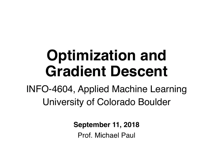
Optimization and Gradient Descent INFO-4604, Applied Machine - PowerPoint PPT Presentation

Optimization and Gradient Descent INFO-4604, Applied Machine Learning University of Colorado Boulder September 11, 2018 Prof. Michael Paul

Prediction Functions Remember: a prediction function is the function that predicts what the output should be, given the input.

Prediction Functions Linear regression: f( x ) = w T x + b Linear classification (perceptron): f( x ) = 1, w T x + b ≥ 0 -1, w T x + b < 0 Need to learn what w should be!

Learning Parameters Goal is to learn to minimize error • Ideally: true error • Instead: training error The loss function gives the training error when using parameters w , denoted L( w ). • Also called cost function • More general: objective function (in general objective could be to minimize or maximize; with loss/cost functions, we want to minimize)

Learning Parameters Goal is to minimize loss function. How do we minimize a function? Let’s review some math.

Rate of Change The slope of a line is also called the rate of change of the line. y = ½ x + 1 “rise” “run”

Rate of Change For nonlinear functions, the “rise over run” formula gives you the average rate of change between two points Average slope from x=-1 to x=0 is: f(x) = x 2 -1

Rate of Change There is also a concept of rate of change at individual points (rather than two points) Slope at x=-1 is: f(x) = x 2 -2

Rate of Change The slope at a point is called the derivative at that point Intuition: f(x) = x 2 Measure the slope between two points that are really close together

Rate of Change The slope at a point is called the derivative at that point Intuition: Measure the slope between two points that are really close together f(x + c) – f(x) c f(x) f(x+c) Limit as c goes to zero

Maxima and Minima Whenever there is a peak in the data, this is a maximum The global maximum is the highest peak in the entire data set, or the largest f(x) value the function can output A local maximum is any peak, when the rate of change switches from positive to negative

Maxima and Minima Whenever there is a trough in the data, this is a minimum The global minimum is the lowest trough in the entire data set, or the smallest f(x) value the function can output A local minimum is any trough, when the rate of change switches from negative to positive

Maxima and Minima From:&https://www.mathsisfun.com/algebra/functions8maxima8minima.html All global maxima and minima are also local maxima and minima

Derivatives The derivative of f(x) = x 2 is 2x Other ways of writing this: f’(x) = 2x d/dx [x 2 ] = 2x df/dx = 2x The derivative is also a function! It depends on the value of x. • The rate of change is different at different points

Derivatives The derivative of f(x) = x 2 is 2x f(x) f’(x)

Derivatives How to calculate a derivative? • Not going to do it in this class. Some software can do it for you. • Wolfram Alpha

Derivatives What if a function has multiple arguments? Ex: f(x 1 , x 2 ) = 3x 1 + 5x 2 df/dx 1 = 3 + 5x 2 The derivative “with respect to” x 1 df/dx 2 = 3x 1 + 5 The derivative “with respect to” x 2 These two functions are called partial derivatives . The vector of all partial derivatives for a function f is called the gradient of the function: ∇ f(x 1 , x 2 ) = < df/dx 1 , df/dx 2 >

From:&http://mathinsight.org/directional_derivative_gradient_introduction

From:&http://mathinsight.org/directional_derivative_gradient_introduction

From:&http://mathinsight.org/directional_derivative_gradient_introduction

Finding Minima The derivative is zero at any local maximum or minimum.

Finding Minima The derivative is zero at any local maximum or minimum. One way to find a minimum: set f’(x)=0 and solve for x. f(x) = x 2 f’(x) = 2x f’(x) = 0 when x = 0, so minimum at x = 0

Finding Minima The derivative is zero at any local maximum or minimum. One way to find a minimum: set f’(x)=0 and solve for x. • For most functions, there isn’t a way to solve this. • Instead: algorithmically search different values of x until you find one that results in a gradient near 0.

Finding Minima If the derivative is positive, the function is increasing. • Don’t move in that direction, because you’ll be moving away from a trough. If the derivative is negative, the function is decreasing. • Keep going, since you’re getting closer to a trough

Finding Minima f’(-1) = -2 At x=-1, the function is decreasing as x gets larger. This is what we want, so let’s make x larger. Increase x by the size of the gradient: -1 + 2 = 1

Finding Minima f’(-1) = -2 At x=-1, the function is decreasing as x gets larger. This is what we want, so let’s make x larger. Increase x by the size of the gradient: -1 + 2 = 1

Finding Minima f’(1) = 2 At x=1, the function is increasing as x gets larger. This is not what we want, so let’s make x smaller. Decrease x by the size of the gradient: 1 - 2 = -1

Finding Minima f’(1) = 2 At x=1, the function is increasing as x gets larger. This is not what we want, so let’s make x smaller. Decrease x by the size of the gradient: 1 - 2 = -1

Finding Minima We will keep jumping between the same two points this way. We can fix this be using a learning rate or step size.

Finding Minima f’(-1) = -2 x += 2 η =

Finding Minima f’(-1) = -2 x += 2 η = Let’s use η = 0.25.

Finding Minima f’(-1) = -2 x = -1 + 2(.25) = -0.5

Finding Minima f’(-1) = -2 x = -1 + 2(.25) = -0.5 f’(-0.5) = -1 x = -0.5 + 1(.25) = -0.25

Finding Minima f’(-1) = -2 x = -1 + 2(.25) = -0.5 f’(-0.5) = -1 x = -0.5 + 1(.25) = -0.25 f’(-0.25) = -0.5 x = -0.25 + 0.5(.25) = -0.125

Finding Minima f’(-1) = -2 x = -1 + 2(.25) = -0.5 f’(-0.5) = -1 x = -0.5 + 1(.25) = -0.25 f’(-0.25) = -0.5 x = -0.25 + 0.5(.25) = -0.125 Eventually we’ll reach x=0.

Gradient Descent 1. Initialize the parameters w to some guess (usually all zeros, or random values) 2. Update the parameters: w = w – η ∇ L( w ) 3. Update the learning rate η (How? Later…) 4. Repeat steps 2-3 until ∇ L( w ) is close to zero.

Gradient Descent Gradient descent is guaranteed to eventually find a local minimum if: • the learning rate is decreased appropriately; • a finite local minimum exists (i.e., the function doesn’t keep decreasing forever).

Gradient Ascent What if we want to find a local maximum ? Same idea, but the update rule moves the parameters in the opposite direction: w = w + η ∇ L( w )

Learning Rate In order to guarantee that the algorithm will converge, the learning rate should decrease over time. Here is a general formula. At iteration t: η t = c 1 / (t a + c 2 ), where 0.5 < a < 2 c1 > 0 c2 ≥ 0

Stopping Criteria For most functions, you probably won’t get the gradient to be exactly equal to 0 in a reasonable amount of time. Once the gradient is sufficiently close to 0 , stop trying to minimize further. How do we measure how close a gradient is to 0 ?

Distance A special case is the distance between a point and zero (the origin ). k d( p , 0 ) = √ (p i ) 2 i=1 This is called the Euclidean norm of p • A norm is a measure of a vector’s length • The Euclidean norm is also called the L2 norm

Distance A special case is the distance between a point and zero (the origin ). k d( p , 0 ) = √ (p i ) 2 i=1 Also written: || p ||

Stopping Criteria Stop when the norm of the gradient is below some threshold, θ : || ∇ L( w )|| < θ Common values of θ are around .01, but if it is taking too long, you can make the threshold larger.

Gradient Descent 1. Initialize the parameters w to some guess (usually all zeros, or random values) 2. Update the parameters: w = w – η ∇ L( w ) η = c 1 / (t a + c 2 ) 3. Repeat step 2 until || ∇ L( w )|| < θ or until the maximum number of iterations is reached.

Revisiting Perceptron In perceptron, you increase the weights if they were an underestimate and decrease if they were an overestimate. w j += η (y i – f(x i )) x ij This looks similar to the gradient descent rule. • Is it? We’ll come back to this.

Adaline Similar algorithm to perceptron (but uncommon): Predictions use the same function: f( x ) = 1, w T x ≥ 0 -1, w T x < 0 (here the bias b is folded into the weight vector w )

Adaline Perceptron minimizes the number of errors. Adaline instead tries to make w T x close to the correct value (1 or -1, even though w T x can be any real number). Loss function for Adaline: N L( w ) = (y i – w T x i ) 2 This is called the squared error . i=1 (This is the same loss function used for linear regression.)

Adaline What is the derivative of the loss? N L( w ) = (y i – w T x i ) 2 i=1 N dL/dw j = -2 x ij (y i – w T x i ) i=1

Adaline The gradient descent algorithm for Adaline updates each feature weight using the rule: N 2 x ij (y i – w T x i ) w j += η i=1 Two main differences from perceptron: • (y i – w T x i ) is a real value, instead of a binary value (perceptron either correct or incorrect) • The update is based on the entire training set, instead of one instance at a time.