OPTIMISING ASSOCIATION RULE ALGORITHMS USING ITEMSET ORDERING - PowerPoint PPT Presentation

OPTIMISING ASSOCIATION RULE ALGORITHMS USING ITEMSET ORDERING ES2001 Peterhouse College, Cambridge Frans Coenen, Paul Leng and Graham Goulbourne The Department of Computer Science The University of Liverpool

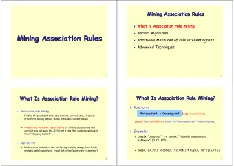
Introduction: The archetypal problem --- shopping basket analysis Which items tend to occur together in shopping baskets? – Examine database of purchase transactions – look for associations Find Association Rules : PQ -> X When P and Q occur together, X is likely to occur also

Support and Confidence • The support support for a rule A for a rule A- ->B is the number (proportion) >B is the number (proportion) of cases in which AB occur together of cases in which AB occur together • The • The confidence confidence for a rule is the ratio of support for rule for a rule is the ratio of support for rule to support for its antecedent to support for its antecedent • The problem: The problem: Find all rules for which support and Find all rules for which support and • confidence exceed some threshold (the frequent frequent sets) sets) confidence exceed some threshold (the ) is the difficult part (confidence follows ) • Support Support is the difficult part (confidence follows •

Lattice of attribute-subsets A B C D AB AC AD BC BD CD BCD ABC ABD ACD ABCD

Apriori Algorithm • Breadth-first lattice traversal: – on each iteration k, examine a Candidate Set C k of sets of k attributes: – Count the support for all members of C k (one pass of the database, requiring all k-subsets of each record to be examined) – Find the set L k of sets with required support – Use this to determine C k+1 , the set of sets of size k+1 all of whose subsets are in L k

Performance • Requires x+1 database passes (where x is the size of the largest frequent set) • Candidate sets can become very large (especially if database is dense) • Examining k-subsets of a record to identify all members of C k present is time-consuming • So: unsatisfactory for databases with densely-packed records

Computing support via Partial support totals • Use a single database pass to count the sets present (not subsets): this gives us m ’ partial support-counts (m ’ < m, the database size) • Use this set of counts to compute the total support for subsets • Gains when records duplicated (m ’ << m) • More important: allows us to reorganise data for efficient computation

Building the tree • For each record i in database: – find the set i on the tree; – increment support-count for all sets on path to i – if set not present on tree, create a node for it • Tree is built dynamically (size ~m rather than 2 n ) • Building tree has already counted support deriving from successor-supersets (leading to interim support-count Q i )

Set enumeration tree: The P-tree A B C D 8 4 2 1 AB AC AD BC BD CD 1 1 4 2 2 1 BCD ACD A BD 1 1 B CD C ABC ABC ABD 1 2 D ABD AB ACD ABCD 1 AC BCD AD ABCD BC

Set enumeration tree: The P-tree A B C D 7 4 2 1 AB AC AD BC BD CD 1 1 3 2 2 1 BCD ACD A BD 1 1 B CD C ABC ABCD ABD 1 3 D ABD AB ACD AC BCD AD ABCD BC

Dummy Nodes A 7 ABC ABCD AC AD 1 3 3 2 ACD A 1 AC AD ABCD ABD 1 3 ABC ABD ACD ABCD

A Dummy Nodes AC A 7 AD ABC ABD AC AD ABC 1 2 1 2 ABD ACD ACD 1 ABCD A ABCD 7 1 AB AC AD 1 2 3 ACD ABC ABD 1 2 1 ABCD 1

Calculating total support A B C D 8 4 2 1 AB AC AD BC BD CD 1 1 4 2 2 1 BCD ACD 1 1 ABC ABD 1 2 i TS = i PS + sum(predessessor nodes of I PS ) ABCD 1 B TS = B PS +AB PS

Calculating total support A B C D 8 4 2 1 AB AC AD BC BD CD 1 1 4 2 2 1 BCD ACD 1 1 D TS = D PS + CD PS + BD PS + BCD PS + ABC ABD 1 2 AD PS + ACD PS + ABD PS + ABCD 1 ABCD PS

Calculating total support A B C D 8 4 2 1 AB AC AD BC BD CD 1 1 4 2 2 1 BCD ACD 1 1 D TS = D PS + CD PS + BD PS + BCD PS + ABC ABD 1 2 AD PS + ACD PS + ABD PS + ABCD 1 ABCD PS

Computing total supports: The T-tree C D A B AB AC BC AD BD CD ABD ACD BCD ABC ABCD

Itemset Ordering • Advantages gained from partial computation is not equally distributed throughout the set of candidates. • For candidate early in the lexicographic order most of the support calculation is complete • If we know the frequency of single items sets we can order the tree so that the most common item sets appear first and thus reduced the effort required for total support counting.

Set enumeration tree: The P-tree A B CD D 3 4 2 1 AB ACD AD BCD BD 1 1 2 1 2 D CD BD ABCD ABD AD 1 1 BCD ACD ABD ABCD

Computing Total Supports • Have already computed interim support Q i for set i • Total support = (adding support for predecessor-supersets) ∑ + Q P i j

Example A B C D AB AC AD BC BD CD BCD ACD ABC ABD ABCD - To complete total for BC, need to add support stored at ABC

General summation algorithm • For each node j in tree: – for all sets i in Target set T: • if i is a subset of j and i is not a subset of the parent of j, add Q j to total for i

Example (2) A B C D AB AC AD BC BD CD BCD ACD ABC ABD ABCD -A dd support stored at ABC to support for AC, BC and C - No need to add to A, AB (already counted) or to B (will have AB added, including ABC)

Modified algorithm • Problem: still have 2 n Totals to count – So use Apriori type algorithm • Count C 1 , C 2 etc in repeated passes of tree

Algorithm Apriori-TFP (Total- from -Partial) • For each node j in P-tree: – i is attribute not in parent node – starting at node i of T-tree: • walk the tree until (parent of) node j is reached, adding support to all subsets of j at the required level • On completion, prune the tree to remove unsupported sets • Generate the next level and repeat

Illustration C D A B AB AC BC AD BD CD ABD ACD BCD ABC ABD ABCD Pass 1: C not supported, so do not add AC,BC,CD to tree Pass2: (eg) Item ABD from P-tree added to AD and BD (tree is walked from D to BD)

Advantages • 1. Duplication in records reduces size of tree • 2. Fewer subsets to be counted: eg, for a record of r attributes, Apriori counts r(r-1)/2 subset-pairs; our method only r-1 • 3. T-tree provides an efficient localisation of candidates to be updated in Apriori-TFP

Related Work • The FP-tree (Han et al.), developed contemporaneously, has similar properties, but: – FP-tree stores a single item only at each node (so more nodes) – FP-tree builds in more links to implement FP- growth algorithm – Conversely, P-tree is generic: Apriori-TFP is only one possible algorithm

Experimental results (1) • Size and construction time for P-tree: – almost independent of N (number of attributes) – scale linearly with M (number of records) – seems to scale linearly as database density increases – less than for FP-tree (because of more nodes and links in latter)

Experimental results (2): time to produce all frequent sets T25.I10.N1K.D10K

Continuing work • Optimise using item ordering heuristic: (as used in FP-growth) • Explore other algorithms (eg Partition) applied to P-tree • Hybrid methods, using different algorithms for subtrees – (exhaustive methods may be effective for small very densely-populated subtrees)