Bayesian Methods David S. Rosenberg New York University March 20, - PowerPoint PPT Presentation
Bayesian Methods David S. Rosenberg New York University March 20, 2018 David S. Rosenberg (New York University) DS-GA 1003 / CSCI-GA 2567 March 20, 2018 1 / 38 Contents Classical Statistics 1 Bayesian Statistics: Introduction 2
Bayesian Methods David S. Rosenberg New York University March 20, 2018 David S. Rosenberg (New York University) DS-GA 1003 / CSCI-GA 2567 March 20, 2018 1 / 38
Contents Classical Statistics 1 Bayesian Statistics: Introduction 2 Bayesian Decision Theory 3 Summary 4 David S. Rosenberg (New York University) DS-GA 1003 / CSCI-GA 2567 March 20, 2018 2 / 38
Classical Statistics David S. Rosenberg (New York University) DS-GA 1003 / CSCI-GA 2567 March 20, 2018 3 / 38
Parametric Family of Densities A parametric family of densities is a set { p ( y | θ ) : θ ∈ Θ } , where p ( y | θ ) is a density on a sample space Y , and θ is a parameter in a [finite dimensional] parameter space Θ . This is the common starting point for a treatment of classical or Bayesian statistics. David S. Rosenberg (New York University) DS-GA 1003 / CSCI-GA 2567 March 20, 2018 4 / 38
Density vs Mass Functions In this lecture, whenever we say “density”, we could replace it with “mass function.” Corresponding integrals would be replaced by summations. (In more advanced, measure-theoretic treatments, they are each considered densities w.r.t. different base measures.) David S. Rosenberg (New York University) DS-GA 1003 / CSCI-GA 2567 March 20, 2018 5 / 38
Frequentist or “Classical” Statistics Parametric family of densities { p ( y | θ ) | θ ∈ Θ } . Assume that p ( y | θ ) governs the world we are observing, for some θ ∈ Θ . If we knew the right θ ∈ Θ , there would be no need for statistics. Instead of θ , we have data D : y 1 ,..., y n sampled i.i.d. p ( y | θ ) . Statistics is about how to get by with D in place of θ . David S. Rosenberg (New York University) DS-GA 1003 / CSCI-GA 2567 March 20, 2018 6 / 38
Point Estimation One type of statistical problem is point estimation . A statistic s = s ( D ) is any function of the data. A statistic ˆ θ = ˆ θ ( D ) taking values in Θ is a point estimator of θ . A good point estimator will have ˆ θ ≈ θ . David S. Rosenberg (New York University) DS-GA 1003 / CSCI-GA 2567 March 20, 2018 7 / 38
Desirable Properties of Point Estimators Desirable statistical properties of point estimators: Consistency: As data size n → ∞ , we get ˆ θ n → θ . Efficiency: (Roughly speaking) ˆ θ n is as accurate as we can get from a sample of size n . Maximum likelihood estimators are consistent and efficient under reasonable conditions. David S. Rosenberg (New York University) DS-GA 1003 / CSCI-GA 2567 March 20, 2018 8 / 38
The Likelihood Function Consider parametric family { p ( y | θ ) : θ ∈ Θ } and i.i.d. sample D = ( y 1 ,..., y n ) . The density for sample D for θ ∈ Θ is n � p ( D | θ ) = p ( y i | θ ) . i = 1 p ( D | θ ) is a function of D and θ . For fixed θ , p ( D | θ ) is a density function on Y n . For fixed D , the function θ �→ p ( D | θ ) is called the likelihood function: L D ( θ ) := p ( D | θ ) . David S. Rosenberg (New York University) DS-GA 1003 / CSCI-GA 2567 March 20, 2018 9 / 38
Maximum Likelihood Estimation Definition The maximum likelihood estimator (MLE) for θ in the model { p ( y , θ ) | θ ∈ Θ } is ˆ θ MLE = argmax L D ( θ ) . θ ∈ Θ Maximum likelihood is just one approach to getting a point estimator for θ . Method of moments is another general approach one learns about in statistics. Later we’ll talk about MAP and posterior mean as approaches to point estimation. These arise naturally in Bayesian settings. David S. Rosenberg (New York University) DS-GA 1003 / CSCI-GA 2567 March 20, 2018 10 / 38
Coin Flipping: Setup Parametric family of mass functions: p ( Heads | θ ) = θ , for θ ∈ Θ = ( 0 , 1 ) . Note that every θ ∈ Θ gives us a different probability model for a coin. David S. Rosenberg (New York University) DS-GA 1003 / CSCI-GA 2567 March 20, 2018 11 / 38
Coin Flipping: Likelihood function Data D = ( H , H , T , T , T , T , T , H ,..., T ) n h : number of heads n t : number of tails Assume these were i.i.d. flips. Likelihood function for data D : L D ( θ ) = p ( D | θ ) = θ n h ( 1 − θ ) n t This is the probability of getting the flips in the order they were received. David S. Rosenberg (New York University) DS-GA 1003 / CSCI-GA 2567 March 20, 2018 12 / 38
Coin Flipping: MLE As usual, easier to maximize the log-likelihood function: ˆ argmax log L D ( θ ) θ MLE = θ ∈ Θ = argmax [ n h log θ + n t log ( 1 − θ )] θ ∈ Θ First order condition: n h n t θ − = 0 1 − θ n h ⇐ ⇒ θ = . n h + n t So ˆ θ MLE is the empirical fraction of heads. David S. Rosenberg (New York University) DS-GA 1003 / CSCI-GA 2567 March 20, 2018 13 / 38
Bayesian Statistics: Introduction David S. Rosenberg (New York University) DS-GA 1003 / CSCI-GA 2567 March 20, 2018 14 / 38
Bayesian Statistics Introduces a new ingredient: the prior distribution. A prior distribution p ( θ ) is a distribution on parameter space Θ . A prior reflects our belief about θ , before seeing any data .. David S. Rosenberg (New York University) DS-GA 1003 / CSCI-GA 2567 March 20, 2018 15 / 38
A Bayesian Model A [parametric] Bayesian model consists of two pieces: A parametric family of densities 1 { p ( D | θ ) | θ ∈ Θ } . A prior distribution p ( θ ) on parameter space Θ . 2 Putting pieces together, we get a joint density on θ and D : p ( D , θ ) = p ( D | θ ) p ( θ ) . David S. Rosenberg (New York University) DS-GA 1003 / CSCI-GA 2567 March 20, 2018 16 / 38
The Posterior Distribution The posterior distribution for θ is p ( θ | D ) . Prior represents belief about θ before observing data D . Posterior represents the rationally “updated” belief about θ , after seeing D . David S. Rosenberg (New York University) DS-GA 1003 / CSCI-GA 2567 March 20, 2018 17 / 38
Expressing the Posterior Distribution By Bayes rule, can write the posterior distribution as p ( θ | D ) = p ( D | θ ) p ( θ ) . p ( D ) Let’s consider both sides as functions of θ , for fixed D . Then both sides are densities on Θ and we can write p ( θ | D ) ∝ p ( D | θ ) p ( θ ) . � �� � � �� � ���� posterior likelihood prior Where ∝ means we’ve dropped factors independent of θ . David S. Rosenberg (New York University) DS-GA 1003 / CSCI-GA 2567 March 20, 2018 18 / 38
Coin Flipping: Bayesian Model Parametric family of mass functions: p ( Heads | θ ) = θ , for θ ∈ Θ = ( 0 , 1 ) . Need a prior distribution p ( θ ) on Θ = ( 0 , 1 ) . A distribution from the Beta family will do the trick... David S. Rosenberg (New York University) DS-GA 1003 / CSCI-GA 2567 March 20, 2018 19 / 38
Coin Flipping: Beta Prior Prior: Beta ( α , β ) θ ∼ θ α − 1 ( 1 − θ ) β − 1 p ( θ ) ∝ Figure by Horas based on the work of Krishnavedala (Own work) [Public domain], via Wikimedia Commons http://commons.wikimedia.org/wiki/File:Beta_distribution_pdf.svg . David S. Rosenberg (New York University) DS-GA 1003 / CSCI-GA 2567 March 20, 2018 20 / 38
Coin Flipping: Beta Prior Prior: θ ∼ Beta ( h , t ) θ h − 1 ( 1 − θ ) t − 1 p ( θ ) ∝ Mean of Beta distribution: h E θ = h + t Mode of Beta distribution: h − 1 argmax p ( θ ) = h + t − 2 θ for h , t > 1. David S. Rosenberg (New York University) DS-GA 1003 / CSCI-GA 2567 March 20, 2018 21 / 38
Coin Flipping: Posterior Prior: θ ∼ Beta ( h , t ) θ h − 1 ( 1 − θ ) t − 1 p ( θ ) ∝ Likelihood function L ( θ ) = p ( D | θ ) = θ n h ( 1 − θ ) n t Posterior density: p ( θ | D ) ∝ p ( θ ) p ( D | θ ) θ h − 1 ( 1 − θ ) t − 1 × θ n h ( 1 − θ ) n t ∝ θ h − 1 + n h ( 1 − θ ) t − 1 + n t = David S. Rosenberg (New York University) DS-GA 1003 / CSCI-GA 2567 March 20, 2018 22 / 38
Posterior is Beta Prior: ∼ Beta ( h , t ) θ θ h − 1 ( 1 − θ ) t − 1 p ( θ ) ∝ Posterior density: θ h − 1 + n h ( 1 − θ ) t − 1 + n t p ( θ | D ) ∝ Posterior is in the beta family : θ | D ∼ Beta ( h + n h , t + n t ) Interpretation : Prior initializes our counts with h heads and t tails. Posterior increments counts by observed n h and n t . David S. Rosenberg (New York University) DS-GA 1003 / CSCI-GA 2567 March 20, 2018 23 / 38
Sidebar: Conjugate Priors Interesting that posterior is in same distribution family as prior. Let π be a family of prior distributions on Θ . Let P parametric family of distributions with parameter space Θ . Definition A family of distributions π is conjugate to parametric model P if for any prior in π , the posterior is always in π . The beta family is conjugate to the coin-flipping (i.e. Bernoulli) model. The family of all probability distributions is conjugate to any parametric model. [Trivially] David S. Rosenberg (New York University) DS-GA 1003 / CSCI-GA 2567 March 20, 2018 24 / 38
Example: Coin Flipping - Concrete Example Suppose we have a coin, possibly biased ( parametric probability model ): p ( Heads | θ ) = θ . Parameter space θ ∈ Θ = [ 0 , 1 ] . Prior distribution: θ ∼ Beta ( 2 , 2 ) . David S. Rosenberg (New York University) DS-GA 1003 / CSCI-GA 2567 March 20, 2018 25 / 38
Example: Coin Flipping Next, we gather some data D = { H , H , T , T , T , T , T , H ,..., T } : Heads: 75 Tails: 60 ˆ 75 θ MLE = 75 + 60 ≈ 0 . 556 Posterior distribution: θ | D ∼ Beta ( 77 , 62 ) : David S. Rosenberg (New York University) DS-GA 1003 / CSCI-GA 2567 March 20, 2018 26 / 38
Recommend
More recommend
Explore More Topics
Stay informed with curated content and fresh updates.


