Optimal sampling of multiple linear processes over a shared medium - PowerPoint PPT Presentation
Optimal sampling of multiple linear processes over a shared medium Sebin Mathew a , Karl H. Johannson b , Aditya Mahajan a IEEE Conference on Decision and Control 17 December, 2018 a McGill University b KTH Royal Institute of Technology Sampling
Optimal sampling of multiple linear processes over a shared medium Sebin Mathew a , Karl H. Johannson b , Aditya Mahajan a IEEE Conference on Decision and Control 17 December, 2018 a McGill University b KTH Royal Institute of Technology
Sampling over shared medium–(Mathew, Johannson, Mahajan) 1 Many remote estimation applications where: Multiple sensors transmit over shared links Link capacity varies exogenously
Sampling over shared medium–(Mathew, Johannson, Mahajan) 1 Sensor Networks Many remote estimation applications where: Multiple sensors transmit over shared links Link capacity varies exogenously
Sampling over shared medium–(Mathew, Johannson, Mahajan) 1 Sensor Networks Internet of Things Many remote estimation applications where: Multiple sensors transmit over shared links Link capacity varies exogenously
Sampling over shared medium–(Mathew, Johannson, Mahajan) 1 Sensor Networks Internet of ThingsSmart Cities Many remote estimation applications where: Multiple sensors transmit over shared links Link capacity varies exogenously
Sampling over shared medium–(Mathew, Johannson, Mahajan) 1 Sensor Networks Internet of ThingsSmart Cities Many remote estimation applications where: Multiple sensors transmit over shared links Link capacity varies exogenously Salient features: Adapt transmission rate at sensors to avoid congestion and, at the same time, minimize estimation errors Adaptation should take place in a low complexity and distributed manner
Sampling over shared medium–(Mathew, Johannson, Mahajan) 1 Sensor Networks Internet of ThingsSmart Cities Many remote estimation applications where: Multiple sensors transmit over shared links Link capacity varies exogenously Salient features: Adapt transmission rate at sensors to avoid congestion and, at the same time, minimize estimation errors Adaptation should take place in a low complexity and distributed manner Show that such questions can be answered using dual decomposition theory
Sampling over shared medium–(Mathew, Johannson, Mahajan) Remote ˆ X 1 (t) ˆ X n (t) X 1 (t) Estimator Sampler 2 Sampler Process n ⋮ Process 1 ⋮ Network System Model X n (t)
Sampling over shared medium–(Mathew, Johannson, Mahajan) Estimator dX i (t) = a i X i (t)dt + dW i (t) . Process dynamics X n (t) ˆ X 1 (t) ˆ X n (t) X 1 (t) Remote 2 Sampler Sampler Process n ⋮ Process 1 ⋮ Network System Model {W i (t)} t≥0 is stationary and indep across sensors.
Sampling over shared medium–(Mathew, Johannson, Mahajan) X 1 (t) Sampling process dX i (t) = a i X i (t)dt + dW i (t) . Process dynamics X n (t) ˆ X 1 (t) ˆ X n (t) Estimator 2 Remote Sampler Sampler Process n ⋮ Process 1 ⋮ Network System Model {W i (t)} t≥0 is stationary and indep across sensors. Sensor i samples process i at rate R i = 1/T i .
Sampling over shared medium–(Mathew, Johannson, Mahajan) X n (t) n Network Sampling process dX i (t) = a i X i (t)dt + dW i (t) . Process dynamics X n (t) ˆ X 1 (t) 2 ˆ X 1 (t) Estimator Remote Sampler Sampler Process n ⋮ Process 1 ⋮ Network System Model {W i (t)} t≥0 is stationary and indep across sensors. Sensor i samples process i at rate R i = 1/T i . Rate region ℛ = {(R 1 , . . . , R n ) ∈ ℝ n ≥0 : ∑ i=1 R i ≤ C}
Sampling over shared medium–(Mathew, Johannson, Mahajan) ˆ At other times: dˆ X i (t) = X i (t) . Estimated process n Network Sampling process dX i (t) = a i X i (t)dt + dW i (t) . Process dynamics 2 ˆ X 1 (t) X n (t) X n (t) ⋮ System Model Network ⋮ Process 1 X 1 (t) X i (t)dt Process n Sampler Sampler Remote Estimator {W i (t)} t≥0 is stationary and indep across sensors. Sensor i samples process i at rate R i = 1/T i . Rate region ℛ = {(R 1 , . . . , R n ) ∈ ℝ n ≥0 : ∑ i=1 R i ≤ C} At a sampling time: ˆ X i (t) = a i ˆ
Sampling over shared medium–(Mathew, Johannson, Mahajan) 3 ] − 1 2a i /R i e 2a i /R i −1 i i , then the state process is a If the noise process is a Wiener process with variance σ 2 Example 2 dt when sensor i is sampling at rate R i . X I (t)) 0 1/R i Mean-square error System Performance and Optimization Problem . (X i (t) − ˆ M i (R i ) = R i ∫ Gauss-Markov (or Ornstein-Uhlenbeck) process, and M i (R i ) = σ 2 2a i [
Sampling over shared medium–(Mathew, Johannson, Mahajan) If the noise process is a Wiener process with variance σ 2 ] − 1 2a i /R i e 2a i /R i −1 M″ i 3 i , then the state process is a Example Assumptions 2 dt when sensor i is sampling at rate R i . X I (t)) 0 1/R i Mean-square error System Performance and Optimization Problem . (X i (t) − ˆ M i (R i ) = R i ∫ Gauss-Markov (or Ornstein-Uhlenbeck) process, and M i (R i ) = σ 2 2a i [ (A1) For any sensor i and rate R i > 0 , M i (R i ) is strictly decreasing and convex in R i . (A2) M i (R i ) is twice difgerentiable and there exists a positive constant c i such that i (R i ) ≥ c i for all R i > 0 .
Sampling over shared medium–(Mathew, Johannson, Mahajan) n Assumptions M″ Problem formulation Find rate (R 1 , . . . , R n ) ∈ ℝ n ≥0 to min ∑ 3 i=1 M i (R i ) such that n ∑ i=1 . ] − 1 2a i /R i System Performance and Optimization Problem Mean-square error 1/R i 0 X I (t)) 2 dt when sensor i is sampling at rate R i . Example If the noise process is a Wiener process with variance σ 2 i , then the state process is a i e 2a i /R i −1 (X i (t) − ˆ M i (R i ) = R i ∫ Gauss-Markov (or Ornstein-Uhlenbeck) process, and M i (R i ) = σ 2 2a i [ (A1) For any sensor i and rate R i > 0 , M i (R i ) is strictly decreasing and convex in R i . (A2) M i (R i ) is twice difgerentiable and there exists a positive constant c i such that i (R i ) ≥ c i for all R i > 0 . R i ≤ C .
Sampling over shared medium–(Mathew, Johannson, Mahajan) 4 Solution approach Proposition Under assumptions (A1) and (A2), the optimization problem has a unique solution 1 , . . . , R ∗ n ) . which we denote by 𝐒 ∗ = (R ∗
Sampling over shared medium–(Mathew, Johannson, Mahajan) 4 Solution approach Proposition Under assumptions (A1) and (A2), the optimization problem has a unique solution 1 , . . . , R ∗ n ) . which we denote by 𝐒 ∗ = (R ∗ How do we fjnd 𝐒 ∗ in a distributed manner?
Sampling over shared medium–(Mathew, Johannson, Mahajan) 5 Primal Problem min 𝐒 ∗ ∈ ℝ n ≥0 n ∑ i=1 M i (R i ) s.t. n ∑ i=1 Distributed Solution via Dual Decomposition R i ≤ C
Sampling over shared medium–(Mathew, Johannson, Mahajan) n i=1 ∑ n where L(𝐒, λ) = min Lagrangian Dual i=1 5 ∑ s.t. M i (R i ) i=1 ∑ n ≥0 𝐒 ∗ ∈ ℝ n min Primal Problem Distributed Solution via Dual Decomposition λ∈ ℝ ≥0 L(𝐒, λ) [M i (R i ) + λR i ] − λC R i ≤ C
Sampling over shared medium–(Mathew, Johannson, Mahajan) 5 Dual Decomposition Distributed Solution via Dual Decomposition [Chiang et al 2007] [Low Lapsley 1999] [Kelly et al 1998] i=1 ∑ n where L(𝐒, λ) = min Lagrangian Dual Decomposes into two parts: Network and Sensor i i=1 ∑ n s.t. M i (R i ) i=1 ∑ n ≥0 𝐒 ∗ ∈ ℝ n min Primal Problem λ∈ ℝ ≥0 L(𝐒, λ) [M i (R i ) + λR i ] − λC R i ≤ C
Sampling over shared medium–(Mathew, Johannson, Mahajan) i=1 [Chiang et al 2007] At each sensor i At the network [ ( C − n ∑ R i,k 5 )] + Distributed Solution via Dual Decomposition Dual Decomposition Decomposes into two parts: Network and Sensor i Syncronous Algorithm Network starts with a guess λ 0 . [Low Lapsley 1999] [Kelly et al 1998] At each iteration k = 0, 1, . . . ∑ Primal Problem min 𝐒 ∗ ∈ ℝ n ≥0 n ∑ i=1 M i (R i ) s.t. n i=1 i=1 Lagrangian Dual min where L(𝐒, λ) = n ∑ λ∈ ℝ ≥0 L(𝐒, λ) [M i (R i ) + λR i ] − λC R i ≤ C Pick R i,k to min M i (R i ) + λ k R i,k λ k+1 = λ k − α k
Sampling over shared medium–(Mathew, Johannson, Mahajan) 6 Properties of synchronous algorithm Theorem 1 lim k→∞ (R 1,k , . . . , R n,k ) = 𝐒 ∗ . Under (A1) and (A2), for any initial guess λ 0 and appropriately chosen step sizes α k , k→∞ 𝐒 k ≔ lim
Sampling over shared medium–(Mathew, Johannson, Mahajan) The synchronous algorithm can be implemented as part of the initial handshaking a new sensor comes on board, or a sensor leaves, or Algorithm needs to be rerun when: Large signaling overhead. Drawbacks protocol when the sensors come online. Implementation 6 k→∞ (R 1,k , . . . , R n,k ) = 𝐒 ∗ . lim Theorem 1 Properties of synchronous algorithm the network capacity changes. Under (A1) and (A2), for any initial guess λ 0 and appropriately chosen step sizes α k , k→∞ 𝐒 k ≔ lim
Sampling over shared medium–(Mathew, Johannson, Mahajan) protocol when the sensors come online. Salient feature: The network doesn’t need to know R i,k . It only needs an the network capacity changes. a new sensor comes on board, or a sensor leaves, or Algorithm needs to be rerun when: Large signaling overhead. Drawbacks The synchronous algorithm can be implemented as part of the initial handshaking 6 Implementation k→∞ (R 1,k , . . . , R n,k ) = 𝐒 ∗ . lim Theorem 1 Properties of synchronous algorithm Under (A1) and (A2), for any initial guess λ 0 and appropriately chosen step sizes α k , k→∞ 𝐒 k ≔ lim estimate of ∑ R i , which it can infer from the received packets.
Recommend
More recommend
Explore More Topics
Stay informed with curated content and fresh updates.
