Optimal Online Prediction in Adversarial Environments Peter - PowerPoint PPT Presentation

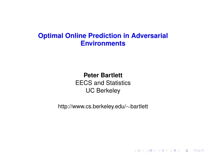
Optimal Online Prediction in Adversarial Environments Peter Bartlett EECS and Statistics UC Berkeley http://www.cs.berkeley.edu/ ∼ bartlett

Online Prediction ◮ Probabilistic Model ◮ Batch : independent random data. ◮ Aim for small expected loss subsequently. ◮ Adversarial Model ◮ Online : Sequence of interactions with an adversary . ◮ Aim for small cumulative loss throughout.

Online Learning: Motivations 1. Adversarial model is appropriate for ◮ Computer security. ◮ Computational finance.

Web Spam Challenge (www.iw3c2.org)

ACM

Online Learning: Motivations 2. Understanding statistical prediction methods. ◮ Many statistical methods, based on probabilistic assumptions , can be effective in an adversarial setting. ◮ Analyzing their performance in adversarial settings provides perspective on their robustness. ◮ We would like violations of the probabilistic assumptions to have a limited impact.

Online Learning: Motivations 3. Online algorithms are also effective in probabilistic settings. ◮ Easy to convert an online algorithm to a batch algorithm. ◮ Easy to show that good online performance implies good i.i.d. performance, for example.

Prediction in Probabilistic Settings ◮ i.i.d. ( X , Y ) , ( X 1 , Y 1 ) , . . . , ( X n , Y n ) from X × Y . ◮ Use data ( X 1 , Y 1 ) , . . . , ( X n , Y n ) to choose f n : X → A with small risk, R ( f n ) = E ℓ ( Y , f n ( X )) .

Online Learning ◮ Repeated game: Player chooses a t Adversary reveals ℓ t ◮ Example: ℓ t ( a t ) = loss ( y t , a t ( x t )) . � ◮ Aim: minimize ℓ t ( a t ) , compared to the best t (in retrospect) from some class: � � regret = ℓ t ( a t ) − min ℓ t ( a ) . a ∈A t t ◮ Data can be adversarially chosen.

Outline 1. An Example from Computational Finance: The Dark Pools Problem. 2. Bounds on Optimal Regret for General Online Prediction Problems.

The Dark Pools Problem ◮ Computational finance: adversarial setting is appropriate. ◮ Online algorithm improves on best known algorithm for probabilistic setting. Joint work with Alekh Agarwal and Max Dama.

Dark Pools Instinet, International Securities Exchange, Chi-X, Investment Technology Group Knight Match, ... (POSIT), ◮ Crossing networks. ◮ Alternative to open exchanges. ◮ Avoid market impact by hiding transaction size and traders’ identities.

Dark Pools

Dark Pools

Dark Pools

Dark Pools

Allocations for Dark Pools The problem: Allocate orders to several dark pools so as to maximize the volume of transactions. ◮ Volume V t must be allocated across K venues: v t 1 , . . . , v t K , such that � K k = 1 v t k = V t . ◮ Venue k can accommodate up to s t k , transacts r t k = min ( v t k , s t k ) . T K � � r t ◮ The aim is to maximize k . t = 1 k = 1

Allocations for Dark Pools: Probabilistic Assumptions Previous work: (Ganchev, Kearns, Nevmyvaka and Wortman, 2008) ◮ Assume venue volumes are i.i.d.: { s t k , k = 1 , . . . , K , t = 1 , . . . , T } . ◮ In deciding how to allocate the first unit, choose the venue k where Pr ( s t k > 0 ) is largest. ◮ Allocate the second and subsequent units in decreasing order of venue tail probabilities. ◮ Algorithm: estimate the tail probabilities (Kaplan-Meier estimator—data is censored), and allocate as if the estimates are correct.

Allocations for Dark Pools: Adversarial Assumptions Why i.i.d. is questionable: ◮ one party’s gain is another’s loss ◮ volume available now affects volume remaining in future ◮ volume available at one venue affects volume available at others In the adversarial setting, we allow an arbitrary sequence of venue capacities ( s t k ), and of total volume to be allocated ( V t ). The aim is to compete with any fixed allocation order.

Continuous Allocations We wish to maximize a sum of (unknown) concave functions of the allocations: T K � � min ( v t k , s t J ( v ) = k ) , t = 1 k = 1 subject to the constraint � K k = 1 v t k ≤ V t . The allocations are parameterized as distributions over the K venues: x 1 t , x 2 t , . . . ∈ ∆ K − 1 = ( K − 1 ) -simplex . Here, x 1 t determines how the first unit is allocated, x 2 t the second, ... V t � The algorithm allocates to the k th venue: v t x v k = t , k . v = 1

Continuous Allocations We wish to maximize a sum of (unknown) concave functions of the distributions: T K � � min ( v t k ( x v t , k ) , s t J = k ) . t = 1 k = 1 Want small regret with respect to an arbitrary distribution x v , and hence w.r.t. an arbitrary allocation. T K � � min ( v t k ( x v k ) , s t regret = k ) − J . t = 1 k = 1

Continuous Allocations We use an exponentiated gradient algorithm: Initialize x v 1 , i = 1 K for v = { 1 , . . . , V } . for t = 1 , . . . , T do k = � V T Set v t v = 1 x v t , k . Receive r t k = min { v t k , s t k } . Set g v t , k = ∇ x v t , k J . Update x v t + 1 , k ∝ x v t , k exp ( η g v t , k ) . end for

Continuous Allocations For all choices of V t ≤ V and of s t Theorem: k , ExpGrad has √ regret no more than 3 V T ln K .

Continuous Allocations For all choices of V t ≤ V and of s t Theorem: k , ExpGrad has √ regret no more than 3 V T ln K . For every algorithm, there are sequences V t and s t Theorem: √ k T ln K / 16. such that regret is at least V

Experimental results Cumulative Reward at Each Round 4 x 10 6 Exp3 3.5 ExpGrad OptKM 3 ParML Cumulative Reward 2.5 2 1.5 1 0.5 0 0 200 400 600 800 1000 1200 1400 1600 1800 2000 Round

Continuous Allocations: i.i.d. data ◮ Simple online-to-batch conversions show ExpGrad obtains per-trial utility within O ( T − 1 / 2 ) of optimal. ◮ Ganchev et al bounds: per-trial utility within O ( T − 1 / 4 ) of optimal.

Discrete allocations ◮ Trades occur in quantized parcels. ◮ Hence, we cannot allocate arbitrary values. ◮ This is analogous to a multi-arm bandit problem: ◮ We cannot directly obtain the gradient at the current x . ◮ But, we can estimate it using importance sampling ideas. Theorem: There is an algorithm for discrete allocation with ex- pected regret ˜ O (( VTK ) 2 / 3 ) . Any algorithm has regret ˜ Ω(( VTK ) 1 / 2 ) .

Dark Pools ◮ Allow adversarial choice of volumes and transactions. ◮ Per trial regret rate superior to previous best known bounds for probabilistic setting. ◮ In simulations, performance comparable to (correct) parametric model’s, and superior to nonparametric estimate.

Outline 1. An Example from Computational Finance: The Dark Pools Problem. 2. Bounds on Optimal Regret for General Online Prediction Problems.

Optimal Regret for General Online Decision Problems ◮ Parallels between probabilistic and online frameworks. ◮ Tools for the analysis of probabilistic problems: Rademacher averages. ◮ Analogous results in the online setting: ◮ Value of dual game. ◮ Bounds in terms of Rademacher averages. ◮ Open problems. Joint work with Jake Abernethy, Alekh Agarwal, Sasha Rakhlin, Karthik Sridharan and Ambuj Tewari.

Prediction in Probabilistic Settings ◮ i.i.d. ( X , Y ) , ( X 1 , Y 1 ) , . . . , ( X n , Y n ) from X × Y . ◮ Use data ( X 1 , Y 1 ) , . . . , ( X n , Y n ) to choose f n : X → A with small risk, R ( f n ) = P ℓ ( Y , f n ( X )) , ideally not much larger than the minimum risk over some comparison class F : excess risk = R ( f n ) − inf f ∈ F R ( f ) .

Parallels between Probabilistic and Online Settings ◮ Prediction with i.i.d. data: ◮ Convex F , strictly convex loss, ℓ ( y , f ( x )) = ( y − f ( x )) 2 : � � ≈ C ( F ) log n P R (ˆ sup f ) − inf f ∈ F R ( f ) . n P ◮ Nonconvex F , or (not strictly) convex loss, ℓ ( y , f ( x )) = | y − f ( x ) | : � � ≈ C ( F ) P R (ˆ sup f ) − inf f ∈ F R ( f ) √ n . P ◮ Online convex optimization: ◮ Convex A , strictly convex ℓ t : per trial regret ≈ c log n . n ◮ ℓ t (not strictly) convex: c √ n . per trial regret ≈

Tools for the analysis of probabilistic problems � n For f n = arg min f ∈ F t = 1 ℓ ( Y t , f ( X t )) , � n � 1 � � � R ( f n ) − inf f ∈ F P ℓ ( Y , f ( X )) ≤ 2 sup ℓ ( Y t , f ( X t )) − P ℓ ( Y , f ( X )) � . � � � n � f ∈ F � t = 1 So supremum of empirical process, indexed by F , gives upper bound on excess risk.

Tools for the analysis of probabilistic problems Typically, this supremum is concentrated about � n � 1 � � � P sup ( ℓ ( Y t , f ( X t )) − P ℓ ( Y , f ( X ))) � � n � � f ∈ F � � t = 1 � n � � P ′ 1 � � � ℓ ( Y t , f ( X t )) − ℓ ( Y ′ t , f ( X ′ � � = P sup t )) � � n � � f ∈ F � t = 1 � n � 1 � � � ℓ ( Y t , f ( X t )) − ℓ ( Y ′ t , f ( X ′ � � ≤ E sup ǫ t t )) � � � n � f ∈ F � � t = 1 n � � 1 � � � ≤ 2 E sup ǫ t ℓ ( Y t , f ( X t )) � , � � n � � f ∈ F � t = 1 where ( X ′ t , Y ′ t ) are independent, with same distribution as ( X , Y ) , and ǫ t are independent Rademacher (uniform ± 1) random variables.