Optimal Left and Right Additive Schwarz Preconditioning for Minimal - PowerPoint PPT Presentation

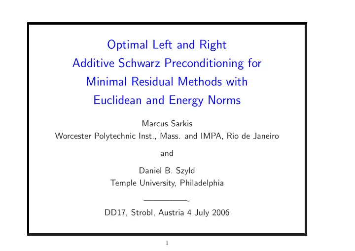
Optimal Left and Right Additive Schwarz Preconditioning for Minimal Residual Methods with Euclidean and Energy Norms Marcus Sarkis Worcester Polytechnic Inst., Mass. and IMPA, Rio de Janeiro and Daniel B. Szyld Temple University, Philadelphia —————- DD17, Strobl, Austria 4 July 2006 1

• We want to solve certain PDEs (non-selfadjoint or indefinit elliptic) discretized by FEM (or divided differences) • Use GMRES (or other Krylov subspace method) • Precondition with Additive Schwarz (with coarse grid correction) • Schwarz methods optimality (energy norm) and Minimal Residuals (2-norm) • Left vs. right preconditioning 2

Examples • Helmholtz equation − ∆ u + cu = f • Advection diffusion equation − ∆ u + b. ∇ u + cu = f • zero Dirichlet b.c. 3

General Problem Statement Solve Bx = f B non-Hermitian, discretization of b ( u, v ) = f ( v ) b ( u, v ) = a ( u, v ) + s ( u, v ) + c ( u, v ) , � a ( u, v ) = ∇ u · ∇ v dx, Ω � b ∈ R d , s ( u, v ) = ( b · ∇ u ) v + ( ∇ · bu ) v dx, Ω � � c ( u, v ) = c uv dx, and f ( v ) = f v dx. Ω Ω Let A be SPD, the discretization of a ( · , · ) . 4

Standard Finite Element Setting Let Ω ⊂ R d , with triangulation T h (Ω) . Let V be the traditional finite element space formed by piecewise linear and continuous functions vanishing on the boundary of Ω . V ⊂ H 1 0 (Ω) . One-to-one correspondence between functions in finite element space and nodal values. We abuse the notation and do not distinguish between them. Let � v � a = a ( v, v ) , and � v � A = ( v T Av ) 1 / 2 be the corresponding norms in V and in R n , respectively. 5

Problem Statement (cont.) • Use Krylov subspace iterative methods (e.g., GMRES) M − 1 Bx = M − 1 f • Left preconditioning: BM − 1 ( Mu ) = f • Right preconditioning: 6

Schwarz Preconditioning Class of Preconditioners based on Domain Decomposition Decomposition of V into a sum of N + 1 subspaces R T i V i ⊂ V , and V = R T 0 V 0 + R T 1 V 1 + · · · + R T N V N . R T i : V i → V extension operator from V i to V . This decomposition usually NOT a direct sum. Subspaces R T i V i , i = 1 , . . . , N are related to a decomposition of the domain Ω into overlapping subregions Ω δ i of size O ( H ) covering Ω . The subspace R T 0 V 0 is the coarse space. 7

Schwarz Preconditioning (cont.) For u i , v i ∈ V i define b i ( u i , v i ) = b ( R T i u i , R T a i ( u i , v i ) = a ( R T i u i , R T i v i ) , i v i ) . Let B i = R i BR T A i = R i AR T i , i be the matrix representations of these local bilinear forms, i.e., the local problems. 8

Two versions of Additive Schwarz Preconditioning here M − 1 = R T 0 B 0 R 0 + � p i B − 1 i =1 R T R i , i or M − 1 = R T 0 B 0 R 0 + � p i =1 R T i A − 1 i R i , where B i = R i BR T i and A i = R i AR T i (local problems) R i restriction, R T i prolongation with overlap δ B 0 coarse problem, size O ( H ) , discretization O ( h ) . 9

Let P = M − 1 B , be the preconditioned problem. Theorem. [Cai and Widlund, 1993] There exist constants H 0 > 0 , c ( H 0 ) > 0 , and C ( H 0 ) > 0 , such that if H ≤ H 0 , then for i = 1 , 2 , and u ∈ V , a ( u, Pu ) a ( u, u ) ≥ c p , and � Pu � a ≤ C p � u � a , where C p = C ( H 0 ) and c p = C − 2 0 c ( H 0 ) . 10

Two-level Schwarz preconditioners are optimal in the sense that bounds for M − 1 B (or BM − 1 ) are independent of the mesh size and the number of subdomains, or slowly varying with them. In our PDEs, we have optimal bounds: ( x, M − 1 Bx ) A � M − 1 Bx � A ≤ C p � x � A . ≥ c p and ( x, x ) A Cai and Zou [NLAA, 2002] observed: Schwarz bounds use energy norms, while GMRES minimizes l 2 norms. Optimality may be lost! (some details in a few slides). 11

GMRES Let v 1 , v 2 , . . . , v m be an orthonormal basis of K m ( M − 1 B, r 0 ) = span { r 0 , M − 1 Br 0 , ( M − 1 B ) 2 r 0 , . . . , ( M − 1 B ) m − 1 r 0 } . x m = arg min {� f − M − 1 Bx � 2 } , x ∈ x 0 + K m ( M − 1 B, r 0 ) • With V m = [ v 1 , v 2 , . . . , v m ] , obtain Arnoldi relation: M − 1 BV m = V m +1 H m +1 ,m H m +1 ,m is ( m + 1) × m upper Hessenberg • Element in K m ( M − 1 B, v 1 ) is a linear combination of v 1 , v 2 , . . . , v m , i.e., of the form V m y , y ∈ R m • Find y = y m and we have x m = x 0 + V m y m � M − 1 f − M − 1 Bx � 2 � M − 1 r 0 − M − 1 BV m y � 2 = = = � V m +1 βe 1 − V m +1 ¯ � βe 1 − ¯ H m y � 2 = H m y � 2 find y using QR factorization of ¯ H m . 12

One convergence bound for GMRES [Elman 1982] (unpreconditioned version) � m/ 2 1 − c 2 � � r m � = � f − Bx m � ≤ � r 0 � , C 2 where ( x, Bx ) � Bx � c = min and C = max . ( x, x ) � x � x � =0 x � =0 13

What Cai and Zou [NLAA, 2002] showed is that for Additive Schwarz M − 1 B is NOT positive real, i.e., there is no c > 0 for which ( x, M − 1 Bx ) ≥ c. ( x, x ) Thus, this GMRES bound cannot be used in this case. We may not have the optimality. 14

Krylov Subspace Methods with Energy Norms Proposed solution: Use GMRES minimizing the A -norm of the residual. [Note: many authors mention this, e.g., Ashby-Manteuffel-Saylor, Essai, Greenbaum, Gutknecht, Weiss, ... ] In this case, we have that M − 1 B is positive real with respect to the A -inner product since ( x, M − 1 Bx ) A � M − 1 Bx � A ≤ C p � x � A . ≥ c p and ( x, x ) A 15

Rework convergence bound for GMRES [Elman 1982] (preconditioned version) � m/ 2 1 − c 2 � � r m � A = � M − 1 f − M − 1 Bx m � A ≤ � M − 1 r 0 � A , C 2 where ( x, M − 1 Bx ) A � Bx � A c = min and C = max . ( x, x ) A � x � A x � =0 x � =0 16

Implementation: Replace each inner product ( x, y ) with ( x, y ) A = x T Ay . Only one matvec with A needed. Basis vectors are A -orthonormal. Arnoldi relation: M − 1 BV m = V m +1 H m +1 . � M − 1 b − M − 1 Bx � A � M − 1 r 0 − M − 1 BV m y � A = = = � V m +1 βe 1 − V m +1 ¯ � βe 1 − ¯ H m y � A = H m y � 2 Same QR factorization of ¯ H m , same code for the minimization. We use this for analysis, but sometimes also valid for computations. 17

Left vs. Right preconditioner For right preconditioner BM − 1 u = f , M − 1 u = x . G = M − T AM − 1 . ( x, x ) A = ( M − 1 u, M − 1 u ) A = ( u, u ) G , • Every left preconditioned system M − 1 Bx = M − 1 f with the A norm is completely equivalent to a right preconditioned system with the M − T AM − 1 -norm. � r 0 − BM − 1 Z m y � M − T AM − 1 � M − 1 r 0 − M − 1 BM − 1 Z m y � A = � βe 1 − ¯ = � βz 1 − M − 1 BV m y � A = H m y � 2 . Z m has the G -orthogonal basis of K m ( r 0 , BM − 1 ) 18

Left vs. Right preconditioner • Converse also holds: for every right preconditioner M with S -norm, this is equivalent to left preconditioning with M using the M T SM -norm. (True in particular for S = I ) • When using the same inner product (norm), left and right preconditioning produce different upper Hessenberg matrices H m . • When using A -inner product for left preconditioning and M − T AM − 1 -inner product for right preconditioning, we have the same upper Hessenberg matrices H m . • Experiments we will show with left preconditioning and A -norm minimization are the same as with right preconditioning with G -norm minimization, G = M − T AM − 1 . 19

Energy Norms vs. ℓ 2 Norm Now, we “have” the optimality with energy norms. What can we say about the ℓ 2 norm? Use equivalence of norms: 1 � � x � 2 ≤ � x � A , � x � A ≤ λ max ( A ) � x � 2 � λ min ( A ) 1 � M − 1 r L � M − 1 r A � M − 1 r A m � 2 ≤ m � 2 ≤ m � A � λ min ( A ) � m/ 2 1 − c 2 � 1 � M − 1 r 0 � A ≤ C 2 � λ min ( A ) � m/ 2 � 1 − c 2 � λ max ( A ) � M − 1 r 0 � 2 ≤ C 2 � λ min ( A ) � m/ 2 1 − c 2 � � � M − 1 r 0 � 2 = κ ( A ) C 2 20

“Asymptotic” Optimality of ℓ 2 Norm � m/ 2 1 − c 2 � � M − 1 r L � � M − 1 r 0 � 2 m � 2 ≤ κ ( A ) C 2 For a fixed mesh size h , Additive Schwarz preconditioned GMRES (2-norm) has a bound that goes to zero at the same speed as the � optimal bound (energy norm), except for a factor κ ( A ) (which of course depends on h ) 21

Numerical Experiments • Helmholtz equation − ∆ u + cu = f , c = − 5 or c = − 120 . • Advection diffusion equation − ∆ u + b. ∇ u + cu = f b T = [10 , 20] , c = 1 , upwind finite differences • both on unit square, zero Dirichlet b.c., f ≡ 1 • Discretization: 64 × 64 ( n = 3969 ), 128 × 128 ( n = 16129 ), or 256 × 256 ( n = 65025 ) nodes p = 4 × 4 or p = 8 × 8 subdomains Overlap: 0 , 1 , 2 (1,3 or 5 lines of nodes) • Tolerance ε = 10 − 8 22

0 2 10 10 −2 0 10 10 Relative G−norm residual Relative l 2 −norm residual −4 −2 10 10 −6 −4 10 10 −8 −6 10 10 −10 −8 10 10 −12 −10 10 10 0 5 10 15 20 25 30 0 5 10 15 20 25 30 Iteration Iteration Figure 1: Helmholtz equation k = − 5 . GMRES minimizing the ℓ 2 norm (o), and the G -norm (*). 64 × 64 grids, 4 × 4 subdomains. δ = 0 Left: G -norm of both residuals. Right: ℓ 2 norm of both residuals. 23