Optical flow Many slides adapted from S. Seitz, R. Szeliski, M. - PowerPoint PPT Presentation
Optical flow Many slides adapted from S. Seitz, R. Szeliski, M. Pollefeys Slides from S. Lazebnik. Motion is a powerful perceptual cue Sometimes, it is the only cue Motion is a powerful perceptual cue Even impoverished motion
Optical flow Many slides adapted from S. Seitz, R. Szeliski, M. Pollefeys Slides from S. Lazebnik.
Motion is a powerful perceptual cue • Sometimes, it is the only cue
Motion is a powerful perceptual cue • Even “impoverished” motion data can evoke a strong percept G. Johansson, “Visual Perception of Biological Motion and a Model For Its Analysis", Perception and Psychophysics 14, 201-211, 1973. Source: L. Lazebnik
Motion is a powerful perceptual cue • Even “impoverished” motion data can evoke a strong percept G. Johansson, “Visual Perception of Biological Motion and a Model For Its Analysis", Perception and Psychophysics 14, 201-211, 1973. Source: L. Lazebnik
Uses of motion in computer vision • 3D shape reconstruction • Object segmentation • Learning and tracking of dynamical models • Event and activity recognition • Self-supervised and predictive learning Source: L. Lazebnik
Motion field • The motion field is the projection of the 3D scene motion into the image Source: L. Lazebnik
Optical flow • Definition : optical flow is the apparent motion of brightness patterns in the image • Ideally, optical flow would be the same as the motion field • Have to be careful: apparent motion can be caused by lighting changes without any actual motion • Think of a uniform rotating sphere under fixed lighting vs. a stationary sphere under moving illumination Source: L. Lazebnik
Estimating optical flow I ( x , y , t –1) I ( x , y , t ) • Given two subsequent frames, estimate the apparent motion field u ( x , y ) and v ( x , y ) between them • Key assumptions • Brightness constancy: projection of the same point looks the same in every frame • Small motion: points do not move very far • Spatial coherence: points move like their neighbors Source: L. Lazebnik
The brightness constancy constraint I ( x , y , t –1) I ( x , y , t ) Brightness Constancy Equation: - = + + I ( x , y , t 1 ) I ( x u , y v ) ( x , y ) ( x , y ), t Linearizing the right side using Taylor expansion: - » + + I ( x , y , t 1 ) I ( x , y , t ) I u ( x , y ) I v ( x , y ) x y + + » I u I v I 0 Hence, x y t Source: L. Lazebnik
The brightness constancy constraint + + = I u I v I 0 x y t • How many equations and unknowns per pixel? • One equation, two unknowns • What does this constraint mean? Ñ × + = I ( u , v ) I 0 t • The component of the flow perpendicular to the gradient (i.e., parallel to the edge) is unknown! Source: L. Lazebnik
The brightness constancy constraint + + = I u I v I 0 x y t • How many equations and unknowns per pixel? • One equation, two unknowns • What does this constraint mean? Ñ × + = I ( u , v ) I 0 t • The component of the flow perpendicular to the gradient (i.e., parallel to the edge) is unknown! gradient ( u , v ) If ( u , v ) satisfies the equation, Ñ × = I ( u ' , v ' ) 0 so does ( u+u’ , v+v’ ) if ( u ’, v ’) ( u + u ’, v + v ’) edge Source: L. Lazebnik
The aperture problem Perceived motion Source: L. Lazebnik
The aperture problem Actual motion Source: L. Lazebnik
The barber pole illusion http://en.wikipedia.org/wiki/Barberpole_illusion Source: L. Lazebnik
The barber pole illusion http://en.wikipedia.org/wiki/Barberpole_illusion Source: L. Lazebnik
Solving the aperture problem • How to get more equations for a pixel? • Spatial coherence constraint: assume the pixel’s neighbors have the same (u,v) • E.g., if we use a 5x5 window, that gives us 25 equations per pixel Ñ × + = I ( x ) [ u , v ] I ( x ) 0 i t i é ù I ( x ) I ( x ) é ù I ( x ) x 1 y 1 t 1 ê ú ê ú I ( x ) I ( x ) é ù u I ( x ) ê ú ê ú x 2 y 2 = - t 2 ê ú ê ú ê ú ! ! ! v ë û ê ú ê ú I ( x ) I ( x ) I ( x ) ê ú ë û ë û x n y n t n B. Lucas and T. Kanade. An iterative image registration technique with an application to stereo vision. In Proceedings of the International Joint Conference on Artificial Intelligence , pp. 674–679, 1981. Source: L. Lazebnik
Lucas-Kanade flow • Linear least squares problem: é ù I ( x ) I ( x ) é ù I ( x ) x 1 y 1 t 1 ê ú ê ú I ( x ) I ( x ) é ù u I ( x ) ê ú ê ú x 2 y 2 = - t 2 ê ú ê ú ê ú ! ! ! v ë û ê ú ê ú I ( x ) I ( x ) I ( x ) ê ú ë û ë û x n y n t n • When is this system solvable? B. Lucas and T. Kanade. An iterative image registration technique with an application to stereo vision. In Proceedings of the International Joint Conference on Artificial Intelligence , pp. 674–679, 1981. Source: L. Lazebnik
Lucas-Kanade flow • Linear least squares problem: é ù I ( x ) I ( x ) é ù I ( x ) x 1 y 1 t 1 = ê ú ê ú A d b I ( x ) I ( x ) é ù u I ( x ) ê ú ê ú x 2 y 2 = - t 2 ê ú ´ ´ ´ ê ú n 2 ê ú 2 1 n 1 ! ! ! v ë û ê ú ê ú I ( x ) I ( x ) I ( x ) ê ú ë û ë û x n y n t n = T T ( A A)d A b • Solution given by å å å M = A T A is the é ù é ù é ù I I I I u I I x x x y = - x t ê ú ê ú ê ú second moment å å å I I I I I I v ê ú ê ú ë û ë û ë û matrix! x y y y y t (summations are over all pixels in the window) B. Lucas and T. Kanade. An iterative image registration technique with an application to stereo vision. In Proceedings of the International Joint Conference on Artificial Intelligence , pp. 674–679, 1981. Source: L. Lazebnik
Recall: second moment matrix • Estimation of optical flow is well-conditioned precisely for regions with high “cornerness”: l 2 “Edge” l 2 >> l 1 “Corner” l 1 and l 2 are large, l 1 ~ l 2 l 1 and l 2 are small “Edge” “Flat” l 1 >> l 2 region l 1 Source: L. Lazebnik
Conditions for solvability • “Bad” case: single straight edge Source: L. Lazebnik
Conditions for solvability • “Good” case Source: L. Lazebnik
Lucas-Kanade flow example Input frames Output Source: MATLAB Central File Exchange Source: L. Lazebnik
Errors in Lucas-Kanade • The motion is large (larger than a pixel) • A point does not move like its neighbors • Brightness constancy does not hold Source: L. Lazebnik
“Flower garden” example Source: L. Lazebnik * From Khurram Hassan-Shafique CAP5415 Computer Vision 2003
“Flower garden” example Lucas-Kanade fails in areas of large motion Source: L. Lazebnik * From Khurram Hassan-Shafique CAP5415 Computer Vision 2003
Multi-resolution estimation Source: L. Lazebnik * From Khurram Hassan-Shafique CAP5415 Computer Vision 2003
Multi-resolution estimation With multi-resolution estimation Source: L. Lazebnik * From Khurram Hassan-Shafique CAP5415 Computer Vision 2003
Fixing the errors in Lucas-Kanade • The motion is large (larger than a pixel) • Multi-resolution estimation, iterative refinement • Feature matching • A point does not move like its neighbors • Motion segmentation J. Wang and E. Adelson, Representing Moving Images with Layers, IEEE Transactions on Image Processing, 1994 Source: L. Lazebnik
Fixing the errors in Lucas-Kanade • The motion is large (larger than a pixel) • Multi-resolution estimation, iterative refinement • Feature matching • A point does not move like its neighbors • Motion segmentation • Brightness constancy does not hold • Feature matching Source: L. Lazebnik
Recommend
More recommend
Explore More Topics
Stay informed with curated content and fresh updates.
