OOPS 2020 Mean field methods in high-dimensional statistics and - PDF document

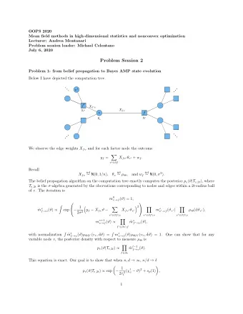
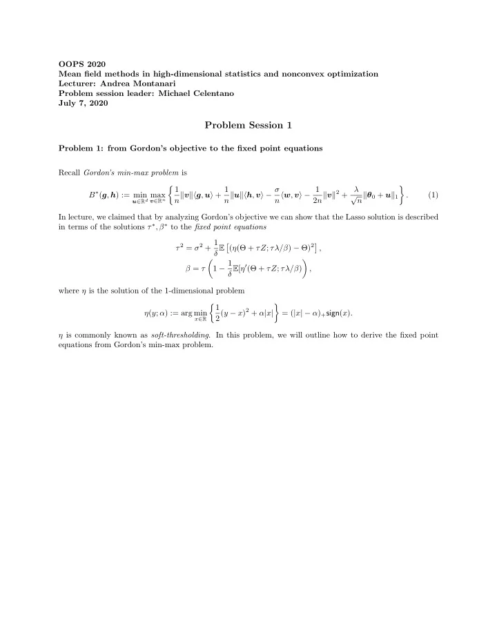
OOPS 2020 Mean field methods in high-dimensional statistics and nonconvex optimization Lecturer: Andrea Montanari Problem session leader: Michael Celentano July 7, 2020 Problem Session 1 Problem 1: from Gordon’s objective to the fixed point equations Recall Gordon’s min-max problem is ⇢ 1 � n k v kh g , u i + 1 n h w , v i � 1 n k u kh h , v i � σ 2 n k v k 2 + λ B ⇤ ( g , h ) := min u 2 R d max p n k θ 0 + u k 1 . (1) v 2 R n In lecture, we claimed that by analyzing Gordon’s objective we can show that the Lasso solution is described in terms of the solutions τ ⇤ , β ⇤ to the fixed point equations ⇥ ( η ( Θ + τ Z ; τλ / β ) � Θ ) 2 ⇤ τ 2 = σ 2 + 1 , δ E ✓ ◆ 1 � 1 δ E [ η 0 ( Θ + τ Z ; τλ / β ) β = τ , where η is the solution of the 1-dimensional problem ⇢ 1 � 2( y � x ) 2 + α | x | η ( y ; α ) := arg min = ( | x | � α ) + sign ( x ) . x 2 R η is commonly known as soft-thresholding . In this problem, we will outline how to derive the fixed point equations from Gordon’s min-max problem.

θ 0 = p n θ 0 and ˜ u = p n u . Prove that B ⇤ ( g , h ) has the same distribution as (a) Define ˜ ⇢✓� � ◆ � � � k ˜ u k � � 1 β � 1 p n � σ w h 2 β 2 + λ � � n k ˜ u 2 R d max min p n p n n h g , u i θ 0 + ˜ u k 1 . (2) � ˜ β � 0 Hint: Let β = k v k / p n

(b) Argue (heuristically) that we may approximate the optimization above by ( r ! ) k ˜ u k 2 + σ 2 � 1 β � 1 2 β 2 + λ n k ˜ u 2 R d max min n h g , u i θ 0 + ˜ u k 1 . (3) n ˜ β � 0 Remark: If we maximize over β � 0 explicitly, we get 8 9 r ! 2 < = u k 2 1 k ˜ + σ 2 � h g , ˜ u i + λ n k ˜ min θ 0 + ˜ u k 1 ; . : 2 n n u 2 ˜ ˜ U + Note that the objective on the right-hand side is locally strongly convex around any point ˜ u at which the first term is positive. When n < p , the Lasso objective is nowhere locally strongly convex. This convenient feature of the new form of Gordon’s problem is very useful for its analysis. We do not explore this further here.

(c) Argue that the quantity in Eq. (3) is equal to ⇢ σ 2 β ⇢ β �� 2 � β 2 2 τ + τβ 2 + 1 u k 2 � β h g , ˜ u i + λ k ˜ 2 τ k ˜ θ 0 + ˜ max β � 0 min n min u k 1 . (4) τ � 0 u 2 R d ˜ � x Hint: Recall the identity p x = min τ � 0 2 τ + τ . 2

(d) Write ⇢ β � u k 2 � β h g , ˜ u i + λ k ˜ u := arg min b 2 τ k ˜ θ 0 + ˜ u k 1 u 2 R d ˜ in terms of the soft-thresholding operator. (e) Compute n o u k 2 � β h g , ˜ β u i + λ k ˜ (i) the derivative of min ˜ 2 τ k ˜ θ 0 + ˜ u k 1 with respect to τ . u 2 R d n o u k 2 � β h g , ˜ β u i + λ k ˜ (ii) the derivative of min ˜ 2 τ k ˜ θ 0 + ˜ u k 1 with respect to β . u 2 R d

(f) Write 1 u k 2 ] and 1 n E [ k b n E [ h g , b u i ] as an expectation over the random variables ( Θ , Z ) ⇠ b µ θ 0 ⌦ N (0 , 1). For the latter, rewrite it using Gaussian integration by parts. (g) Take the derivative of the objective in Eq. (4) with respect to τ and with respect to β . Show that setting the expectations of these derivatives to 0 is equivalent to the fixed point equations.

Problem 2: Gordon’s objective for max-margin classification The use of Gordon’s technique extends well beyond linear models. In logistic regression, we receive iid samples according to y i ⇠ Rad ( f ( h x i , θ 0 i )) , x i ⇠ N (0 , I d ) , exp( x ) f ( x ) = exp( x ) + exp( � x ) . For a certain δ ⇤ > 0 the following occurs: when n/p ! δ < δ ⇤ , n, p ! 1 , with high probability there exists θ such that y i h x i , θ i > 0 for all i = 1 , . . . , n . In such a regime, the data is linearly separable . The max-margin classifier is defined as ⇢ � b θ 2 arg max min i  n y i h x i , θ i : k θ k  1 , (5) θ and the value of the optimization problem, which we denote by κ ( y , X ), is called the maximum margin . To simplify notation, we assume in this problem that k θ 0 k = 1. In this problem, we outline how to set up Gordon’s problem for max-margin classification. The analysis of Gordon’s objective is complicated, and we do not describe it here. See Montanari, Ruan, Sohn, Yan (2019+). “The generalization error of max-margin linear classifiers: High-dimensional asymptotics in the overparameterized regime.” arxiv:1911.01544 .

(a) Show that κ ( y , X ) � κ if and only if k θ k 1 k ( κ 1 � ( y � X θ )) + k 2 = 0 . min Argue that 1 1 λ > ( κ 1 � y � X θ ) p p min k ( κ 1 � ( y � X θ )) + k 2 = min max d d k θ k 1 k θ k 1 k λ k 1 , λ � 0 1 λ > ( κ y � X θ ) . = min max p d k θ k 1 k λ k 1 , λ � y � 0 (b) Why can’t we use Gordon’s inequality to compare the preceding min-max problem to 1 ( κ λ > y + k λ k g > θ + k θ k h > λ )? min max p d k θ k 1 k λ k 1 , y � λ � 0

(c) Let ˜ x = X θ 0 . Show that the min-max problem is equivalent to 1 λ > ( κ 1 � ( y � ˜ min max p x ) h θ 0 , θ i � y � X Π θ ⊥ 0 θ ) . d k θ k 1 k λ k 1 , λ � 0 Here Π θ ⊥ 0 is the projection operator onto the orthogonal complement of the space spaned by θ 0 . Argue that ✓ ◆ 1 λ > ( κ 1 � ( y � ˜ p P min max x ) h θ 0 , θ i � y � X Π θ ⊥ 0 θ )  t d k θ k 1 k λ k 1 , λ � 0 ✓ ◆ ⇣ ⌘ 1 λ > ( κ 1 � ( y � ˜ x ) h θ 0 , θ i ) + k λ k g > Π θ ⊥ 0 θ k h > λ p  2 P min max 0 θ + k Π θ ⊥  t , d k θ k 1 k λ k 1 , λ � 0 and likewise for the comparison of the probabilities that the min-max values exceed t , where g ⇠ N (0 , I d ) and h ⇠ N (0 , I n ) independent of everything else. P n (d) What is the limit in Wasserstein-2 distance of 1 i =1 δ ( y i , ˜ x i ,h i ) ? n