Problem Session 2 Problem 1: from belief propagation to Bayes AMP - PDF document

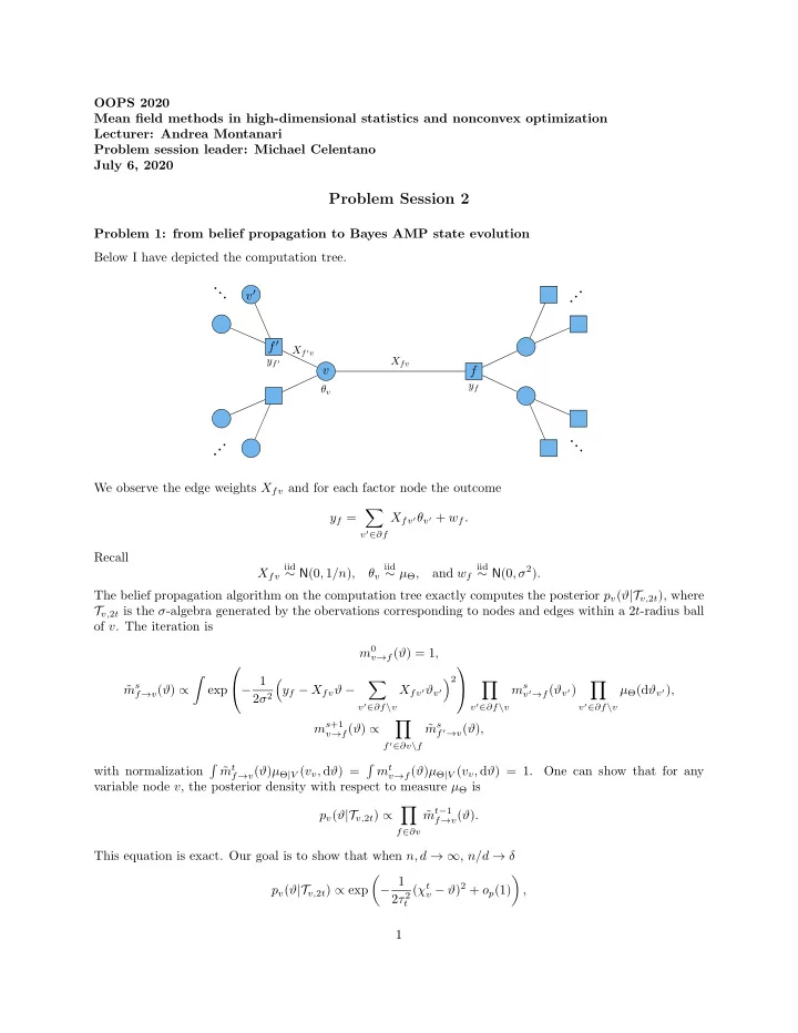
OOPS 2020 Mean field methods in high-dimensional statistics and nonconvex optimization Lecturer: Andrea Montanari Problem session leader: Michael Celentano July 6, 2020 Problem Session 2 Problem 1: from belief propagation to Bayes AMP state evolution Below I have depicted the computation tree. · · · v ′ · · · f ′ X f ′ v y f ′ X fv v f y f θ v · · · · · · We observe the edge weights X fv and for each factor node the outcome � X fv ′ θ v ′ + w f . y f = v ′ ∈ ∂f Recall iid iid iid ∼ N (0 , σ 2 ) . X fv ∼ N (0 , 1 /n ) , θ v ∼ µ Θ , and w f The belief propagation algorithm on the computation tree exactly computes the posterior p v ( ϑ |T v, 2 t ), where T v, 2 t is the σ -algebra generated by the obervations corresponding to nodes and edges within a 2 t -radius ball of v . The iteration is m 0 v → f ( ϑ ) = 1 ,   �  − 1 � 2 � m s � � m s � ˜ f → v ( ϑ ) ∝ exp y f − X fv ϑ − X fv ′ ϑ v ′ v ′ → f ( ϑ v ′ ) µ Θ (d ϑ v ′ ) ,  2 σ 2 v ′ ∈ ∂f \ v v ′ ∈ ∂f \ v v ′ ∈ ∂f \ v � m s +1 m s v → f ( ϑ ) ∝ ˜ f ′ → v ( ϑ ) , f ′ ∈ ∂v \ f � m t � m t with normalization ˜ f → v ( ϑ ) µ Θ | V ( v v , d ϑ ) = v → f ( ϑ ) µ Θ | V ( v v , d ϑ ) = 1. One can show that for any variable node v , the posterior density with respect to measure µ Θ is � m t − 1 p v ( ϑ |T v, 2 t ) ∝ ˜ f → v ( ϑ ) . f ∈ ∂v This equation is exact. Our goal is to show that when n, d → ∞ , n/d → δ � − 1 � v − ϑ ) 2 + o p (1) ( χ t p v ( ϑ |T v, 2 t ) ∝ exp , 2 τ 2 t 1

d where ( χ t v , θ v ) → (Θ + τ t Z, Θ), Θ ∼ µ Θ , G ∼ N (0 , 1) independent of Θ, and τ t is given by the Bayes AMP state evolution equations t +1 = σ 2 + 1 τ 2 δ mmse Θ ( τ 2 t ) , initialized by τ 2 0 = ∞ . In fact, this follows without too much work once we show that � � − 1 v → f − ϑ ) 2 + o p (1) m s ( χ s v → f ( ϑ ) ∝ exp , (1) 2 τ 2 s d where ( χ s → (Θ + τ s Zµ s v → f , θ v ) v ′ → f − , Θ). This problem focuses on establishing (1). We do so inductively. The base case more-or-less follows the standard inductive step, except that we need to pay some attention to the infinite variance τ 2 0 = ∞ . We do not consider the base case here. Throughout, we assume µ Θ has compact support. We do not carefully verify the validity of all approximations. See Celentano, Montanari, Wu. “The estimation error of general first order methods.” COLT 2020 , for complete details. 2

(a) Define � � v → f ) 2 = µ s ϑm s ( τ s ϑ 2 m s v → f ( ϑ ) µ Θ (d ϑ ) − ( µ s v ′ → f ) 2 , v → f = v → f ( ϑ ) µ Θ (d ϑ ) , and f → v ) 2 = � � µ s X fv ′ µ s τ s X 2 fv ′ ( τ s v ′ → f ) 2 . ˜ f → v = v ′ → f , (˜ v ′ ∈ ∂f \ v v ′ ∈ ∂f \ v Argue (non-rigorously) that we may approximate (up to normalization) m s µ s τ s � � ˜ f → v ( ϑ ) ≈ E G p ( X fv ϑ + ˜ f → v + ˜ f → v G − y f ) , 2 σ 2 x 2 is the normal density at variance σ 2 . 1 2 πσ e − 1 where G ∼ N (0 , 1) and p ( x ) = √ v → f ) 2 have a simple statistical interpretation: they are the pos- Remark: The quantities µ s v → f and ( τ s terior mean and variance for θ v given observations in the computation tree within distance 2 s of node v and excluding the branch in the direction of f . (b) Using the inductive hypothesis, show that as n, d → ∞ , n/d → δ → 1 p τ s f → v ) 2 δ mmse Θ ( τ 2 τ 2 (˜ s ) =: ˜ s . f → v = X fv θ v + ˜ µ s Z s Further, note y f − ˜ f → v , where ˜ � Z s X fv ′ ( θ v ′ − µ s f → v = w f + v ′ → f ) . v ′ ∈ ∂f \ v Argue � 0 , σ 2 + 1 � d Z s ˜ δ mmse Θ ( τ 2 → N s ) f → v and is independent of X fv and θ v . v ′ → f ( ϑ v ′ ) as v ′ varies in ∂f are iid and independent of the edge weights Hint: The (random) functions m s X fv ′ . Why? (c) For any smooth probability density f : R → R > 0 , µ ∈ R , and τ > 0, show that d τG )] = − 1 µ log E G [ f (˜ µ + ˜ τ E [ G | S + ˜ τG = ˜ µ ] , d˜ ˜ d 2 τG )] = − 1 µ 2 log E G [ f (˜ µ + ˜ τ 2 (1 − Var[ G | S + ˜ τG = ˜ µ ]) , d˜ ˜ where S ∼ f ( s )d s independent of G ∼ N (0 , 1). (d) We Taylor expand f → v ϑ − 1 f → v ϑ 2 + O p ( n − 3 / 2 ) . fv ˜ m s a s 2 X 2 b s log ˜ f → v ( ϑ ) ≈ const + X fv ˜ f → v and ˜ a s b s (We take this to be the definition of ˜ f → v ). Taking the approximation in part (a) to hold with equality, argue 1 1 ˜ a s µ s b s ˜ f → v = ( y f − ˜ f → v ) + o p (1) , f → v = + o p (1) . τ 2 τ 2 s +1 s +1 3

µ s (e) Taking the approximations in part (d) to hold with equality and using part (b) to subsitute for y f − ˜ f → v , Taylor expand log m s +1 v → f ( ϑ ) to conclude 1 1 ϑ 2 + o p (1) , log m s +1 χ s +1 v → f ( ϑ ) = const + v → f ϑ − τ 2 τ 2 s +1 s +1 d where ( χ s +1 v → f , Θ) → (Θ+ τ s +1 Z, Θ). Why do we expect this Taylor expansion to be valid for all ϑ = O (1)? Conclude Eq. (1). 4