On Hamilton-Jacobi partial differential equation and architectures - PowerPoint PPT Presentation

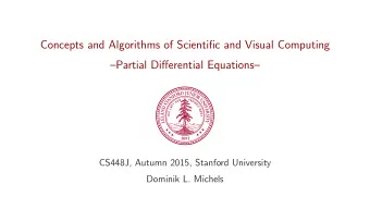
On Hamilton-Jacobi partial differential equation and architectures of neural networks J´ erˆ ome Darbon Division of Applied Mathematics, Brown University ICODE Workshop on numerical solution of HJB equation January 9, 2020 Joint work with Tingwei Meng and Gabriel Provencher Langlois Work supported by NSF DMS 1820821 J. Darbon, ICODE workshop, January 2020 1 / 27

Context and motivation Consider the initial value problem ∂ S  in R n × ( 0 , + ∞ ) ∂ t ( x , t ) + H ( ∇ x S ( x , t ) , x , t ) = ε △ S ( x , t ) ,  ∀ x ∈ R n .  S ( x , 0 ) = J ( x ) Goals: compute the viscosity solution for a given ( x , t ) ∈ R n × [ 0 , + ∞ ) evaluate S ( x , t ) and ∇ x S ( x , t ) very high dimension fast to allow applications requiring real-time computations low memory and low energy for embedded system Pros and cons for computations with grid-based approaches: many advanced and sophisticated numerical schemes (e.g., ENO, WENO, DG) with excellent theoretical properties the number of grid-points is exponential in n → using numerical approximations is not doable for n ≥ 4 J. Darbon, ICODE workshop, January 2020 2 / 27

Overcoming/mitigating the curse of dimensionality Several approaches to mitigate/overcome the curse of differentiability Max-plus methods [Akian, Dower, McEneaney, Flening, Gaubert, Qu . . . ] Tensor decomposition methods [Doglov, Horowitz, Kalise, Kunisch, Todorov, . . . ] Sparse grids [Bokanovski, Garcke, Grieble, Kang, Klompmaker, Kr¨ oner, Wilcox] Model order reduction [Alla, Kunisch, Falcone, Wolkwein, . . . ] Optimization techniques via representation formulas [D., Dower, Osher, Yegerov, . . . ] . . . More recently, there is a significant trend in using Machine Learning and Neural Network techniques for solving PDEs → A key idea is to leverage universal approximation theorems J. Darbon, ICODE workshop, January 2020 3 / 27

Neural Network: a computational point of view Pros and cons of Neural Networks for evaluating solutions It seems to be hard to find Neural Networks that are interpretable, generalizable which yield reproducible results Huge computational advantage dedicated hardware for NN is now available: e.g., Xilinx AI (FPGA + silicon design), Intel AI (FPGA + new CPU assembly instructions), and many other (startup) companies high throughput / low latency (more precise meaning of “fast”) low energy requirement (e.g., a few Watts) → suitable for embedded computing and data centers Can we leverage these computational resources for high-dimensional H-J PDEs? How can we mathematically certify that Neural Networks (NNs) actually computes a viscosity solution of a H-J PDE? ⇒ Establish new connections between NN architectures and representation formulas of H-J PDE solutions → the physics of some H-J PDEs can be encoded by NN architecture → the parameters of the NN define Hamiltonians and initial data → no approximation: exact evaluation of S ( x , t ) and ∇ x S ( x , t ) → suggests an interpretation of some NN architectures in terms of H-J PDEs → does not rely on NN universal approximation theorems J. Darbon, ICODE workshop, January 2020 4 / 27

Outline 1. Shallow NN architectures and representation of solution of H-J PDEs A class of first-order H-J 1 Associated conservation law (1D) 2 A class of second order H-J 3 2. Numerical experiments for solving some inverse problems involving H-J using data and learning/optimization algorithms 3. Suggestions of other NN architectures for other H-J PDEs 4. Some conclusions J. Darbon, ICODE workshop, January 2020 5 / 27

A first shallow network architecture Architecture: fully connected layer followed by the activation function “max-pooling” This network defines a function f : R n × [ 0 , + ∞ ) → R f ( x , t ; { p i , θ i , γ i } m i = 1 ) = i ∈{ 1 ,..., m } {� p i , x � − t θ i − γ i } . max Goal: Find conditions on the parameters such that f satisfies a PDE, and find the PDE J. Darbon, ICODE workshop, January 2020 6 / 27

Assumptions on the parameters Recall: the network f ( x , t ; { p i , θ i , γ i } m i = 1 ) = max i ∈{ 1 ,..., m } {� p i , x � − t θ i − γ i } We adopt the following assumptions on the parameters: (A1) The parameters { p i } m i = 1 are pairwise distinct, i.e., p i � = p j if i � = j . (A2) There exists a convex function g : R n → R such that g ( p i ) = γ i . (A3) For any j ∈ { 1 , . . . , m } and any ( α 1 , . . . , α m ) ∈ R m that satisfy  ( α 1 , . . . , α m ) ∈ ∆ m with α j = 0 ,   � i � = j α i p i = p j ,  � i � = j α i γ i = γ j ,  there holds � i � = j α i θ i > θ j . where ∆ m denotes the unit simplex of dimension m ( A 1 ) and ( A 3 ) are NOT strong assumptions. - ( A 1 ) simplifies the mathematical analysis - ( A 3 ) simply states the each “neuron” should contribute to the definition of f . - If ( A 3 ) is not satisfied, then it means that some neurons can be removed and the NN still defines the same function f J. Darbon, ICODE workshop, January 2020 7 / 27

Define initial data and Hamiltonians from parameters Recall: the network f f ( x , t ; { p i , θ i , γ i } m i = 1 ) = i ∈{ 1 ,..., m } {� p i , x � − t θ i − γ i } max (1) Define the initial data J using the NN parameters { p i , γ i } m i = 1 f ( x , 0 ) = J ( x ) := i ∈{ 1 ,..., m } {� p i , x � − γ i } max (2) Then, J : R n → R is convex, and its Legendre transform J ∗ reads  �� m if p ∈ conv ( { p i } m � min ( α 1 ,...,α m ) ∈ ∆ m i = 1 α i γ i , i = 1 ) ,  J ∗ ( p ) = � m i = 1 α i p i = p + ∞ , otherwise .  Denote by A ( p ) the set of minimizers in the above optimization problem. Define the Hamiltonian H : R n → R ∪ { + ∞} by � �� m if p ∈ dom J ∗ , � inf α ∈A ( p ) i = 1 α i θ i , H ( p ) := (3) + ∞ , otherwise . J. Darbon, ICODE workshop, January 2020 8 / 27

NN computes viscosity solutions Theorem Assume (A1)-(A3) hold. Let f be the neural network defined by Eq. (1) with parameters { ( p i , θ i , γ i ) } m i = 1 . Let J and H be the functions defined in Eqs. (2) and (3), respectively, and let H : R n → R be a continuous function. Then the following two statements hold. ˜ (i) The neural network f is the unique uniformly continuous viscosity solution to the Hamilton–Jacobi equation � ∂ f x ∈ R n , t > 0 , ∂ t ( x , t ) + H ( ∇ x f ( x , t )) = 0 , (4) x ∈ R n . f ( x , 0 ) = J ( x ) , Moreover, f is jointly convex in ( x ,t). (ii) The neural network f is the unique uniformly continuous viscosity solution to the Hamilton–Jacobi equation � ∂ t ( x , t ) + ˜ ∂ f x ∈ R n , t > 0 , H ( ∇ x f ( x , t )) = 0 , (5) x ∈ R n . f ( x , 0 ) = J ( x ) , if and only if ˜ H ( p i ) = H ( p i ) for every i = 1 , . . . , m and ˜ H ( p ) � H ( p ) for every p ∈ dom J ∗ . J. Darbon, ICODE workshop, January 2020 9 / 27

NN computes viscosity solutions The network computes viscosity solution for H and J given by parameters Hamiltonians are not unique. However, among all possible Hamiltonians, H is the smallest one. In addition, ∇ x S ( x , t ) (when it exists) is given by the element that realizes the maximum is the “max-pooling” J. Darbon, ICODE workshop, January 2020 10 / 27

NN computes viscosity solutions: An example Consider J orig ( x ) = � x � ∞ and H orig ( p ) = − � p � 2 for every x , p ∈ R n . 2 2 Denote by e i the i th standard unit vector in R n . Let m = 2 n , { p i } m i = 1 = {± e i } n i = 1 , θ i = − n 2 , and γ i = 0 for every i ∈ { 1 , . . . , m } . The viscosity solution S is given by S ( x , t ) = � x � ∞ + nt i ∈{ 1 ,..., m } {� p i , x � − t θ i − γ i } , for every x ∈ R n and t � 0 . 2 = max Hence, S can be represented using the proposed neural network with parameters { ( p i , − n 2 , 0 ) } m i = 1 . The parameters { ( p i , − n 2 , 0 ) } m i = 1 define the following initial data and smallest Hamiltonian J ( x ) = � x � ∞ , for every x ∈ R n ; � − n 2 , p ∈ B n ; H ( p ) = + ∞ , otherwise , where B n is the unit ball with respect to the l 1 norm in R n , i.e., B n = conv {± e i : i ∈ { 1 , . . . , n }} By Thm. 1, S is a viscosity solution to the HJ PDE (5) if and only if ˜ H ( p i ) = − n 2 for every i ∈ { 1 , . . . , m } and ˜ H ( p ) ≥ − n 2 for every p ∈ B n \ { p i } m i = 1 . Therefore, the Hamiltonian H orig is one candidate satisfying these constraints. J. Darbon, ICODE workshop, January 2020 11 / 27

Architecture for the gradient map This NN architecture computes the spatial gradient of the solution (i.e., the momentum) Consider u : R n × [ 0 , + ∞ ) → R n defined by u ( x , t ) = ∇ x f ( x , t ) = p j , where j ∈ arg max {� p i , x � − t θ i − γ i } . (6) i ∈{ 1 ,..., m } J. Darbon, ICODE workshop, January 2020 12 / 27