On estimation of functional causal models: Post - nonlinear - PowerPoint PPT Presentation
On estimation of functional causal models: Post - nonlinear causal model as an example Kun Zhang, Zhikun W ang, Bernhard Schlkopf Dept. Empirical Inference Max Planck Institute for Intelligent Systems Tbingen, Germany 1
On estimation of � � � � functional causal models: Post - nonlinear causal model as an example Kun Zhang, Zhikun W ang, Bernhard Schölkopf Dept. Empirical Inference Max Planck Institute for Intelligent Systems Tübingen, Germany 1
Causal discovery l Causal discovery: identify causal relations from purely observed data X1 X2 ------------- - 1.1 1.0 ? 2.1 2.0 X 1 X 2 l In the past decades, under certain 3.1 4.2 2.3 - 0.6 assumptions, it was made possible to 1.3 2.2 - 1.8 0.9 derive causation from passively . . . . observed data . . ¡ statistical data ⇒ causal structure ¡ causal Markov assumption ¡ faithfulness… 2
Constraint - based causal discovery • under Markov condition & faithfulness assumption, uses ( conditional ) independence constraints to find candidate causal structures • example: PC algorithm ( Spirtes & Glymour, 1991 ) Y Z | X • Markov equivalence class • pattern Y ⎯ X ⎯ Z • same adjacencies • → if all agree on orientation; ⎯ if disagree • might be unique: v - structure Y Z 3
Constraint - based method: An inverse problem • { local causal structures } → { conditional independences } ∅ Y X Z X Y X Y Z X Y X Y Z X Y Z X Z | Y X Y Z 4
Constraint - based method: An inverse problem • { local causal structures } → { conditional independences } ∅ Y X faithfulness Z X Y X Y Z X Y X Y Z X Y Z X Z | Y X Y Z 4
Constraint - based method: An inverse problem • { local causal structures } → { conditional independences } ∅ Y X faithfulness Z X Y X Y Z X Y equivalence class X Y Z X Y Z X Z | Y X Y Z 4
Constraint - based method: An inverse problem • { local causal structures } → { conditional independences } ∅ Y X faithfulness X Y or two - variable case? Z X Y X Y or X Y Z X Y Z X Y equivalence class X Y Z X Y Z X Z | Y X Y Z 4
Constraint - based method: An inverse problem • { local causal structures } → { conditional independences } ∅ Y X faithfulness X Y or two - variable case? Z X Y X Y or X Y Z X Y Z X Y equivalence class X Y Z • Instead, try to directly X Y Z identify local causal X Z | Y structures with functional causal models X Y Z 4
Outline • Causal discovery based on functional causal models ( FCMs ) • Estimation of FCMs: Relationship between dependence minimization and maximum likelihood • Post - nonlinear causal model as an example: By warped Gaussian processes with flexible noise distribution 5
Causality is about data - generating process X Y f E • Functional causal model Y = f ( X, E ) : E ff ect generated from cause with independent noise • Why useful? • structural constraints on f guarantee identifiability of the causal model, i.e., asymmetry in X and Y • in practice f can usually be approximated with a well - constrained form ! • How to distinguish cause from e ff ect: • Fit the model for both directions, and see which direction gives independence between the assumed cause and noise 6
FCM cannot distinguish cause from e ff ect without constraints on f • Without constraints on f , for given ( X, Y ), both Y = f 1 ( X , E ) with E X and X = f 2 ( X , E 1 ) with E 1 Y are possible • E.g., with a Gram-Schmidt-orthogonalization procedure (Darmois, ‘51, Hyvärinen & Pajunen, ‘99) x = cdf( x 1 ), so ! ! x ~ U (0,1); x 2 # e = cdf( y | ! x ) = x , y ( ! p ! x , t ) dt . !" Then ( x , y ) $ ( ! x , e ), with E _||_ X 7
( Generally ) identifiable FCMs with independent noise • linear non - Gaussian acyclic causal model ( Shimizu et al., ‘06 ) Y = aX +E • additive noise model ( Hoyer et al., ’09 ) Y = f ( X ) +E • post - nonlinear ( PNL ) causal model ( Zhang & Hyvärinen, ’09 ) Y = f 2 ( f 1 ( X ) +E ) Some papers estimate the models by maximum likelihood; some propose to minimize the dependence between X and E: What is the di ff erence? 8
Mutual information minimization vs. maximum likelihood ? • Model: Y = f ( X, E ; θ 1 ); E ⊥ ⊥ X , E ∼ p ( E ; θ 2 ), f ∈ F (appropriately constrained) Independence criterion Maximum likelihood T T E ; θ ) = − 1 X minimizing I ( X, ˆ X maximizing l X → Y ( θ ) = log P F ( x i , y i ) log p ( X = x i ) − T i =1 i =1 T T T 1 X X X = log p ( X = x i ) + log p ( E = ˆ e i ; θ 2 ) − log p ( X = x i , Y = y i )+ T i =1 i =1 i =1 T T T 1 e i ; θ 2 ) + 1 � ∂ f � ∂ f � � � � log p ( ˆ X X X � � E = ˆ log log � . � � � � � � E =ˆ T T ∂ E E =ˆ � e i ∂ E e i i =1 i =1 i =1 T T l X → Y ( θ ) = 1 1 log p ( X = x i , Y = y i ) − I ( X, ˆ X E ; θ ) . T i =1 • Maximum likelihood is equivalent to mutual information minimization • However, convenient to do model selection with maximum likelihood ! 9
Loss that might be caused by a wrongly specified noise distribution Y = f ( X, E ; θ 1 ); E ⊥ ⊥ X , E ∼ p ( E ; θ 2 ), f ∈ F (appropriately constrained) • Maximum likelihood ( or mutual information minimization ) aims to maximize � � J X → Y = P T e i ) − P T � ∂ f � i =1 log p ( E = ˆ i =1 log � � � ∂ E E =ˆ � e i • If f has additive noise, ∂ f / ∂ E ≡ 1 ; reduces to ordinary regression problem • In general, if p ( E ) is wrongly specified ( e.g., simply set to Gaussian ) , the estimated f might not be statistically consistent • The estimated f might have to sacrifice to make the estimated noise closer to the specified p ( E ) such that term 1 becomes bigger; a trade - o ff of the two terms, is maximized 10
Post - nonlinear causal model: An example • Without prior knowledge, the assumed model is expected to be • general enough: adapted to approximate the true generating process • identifiable: asymmetry in causes and e ff ects • post - nonlinear ( PNL ) causal model: Y = f 2 ( f 1 ( X ) + E ) • PNL causal model is generally identifiable ( Zhang & Hyvärinen, ’09 ) 11
Estimating PNL model by Warped Gaussian processes with non-Gaussian noise Y = f 2 ( f 1 ( X ) + E ) • Previously estimated by minimizing mutual information between X and Ê : di ffi cult to do model selection • A maximum likelihood perspective • Using a Gaussian process ( GP ) prior for f 1 ⇒ warped Gaussian processes ( Snelson et al., 2004 ) • Further use a flexible noise distribution ( mixture of Gaussians ) for E ; otherwise the estimated f may be inconsistent • Represent f 2 with some basis functions • Use MCMC for Bayesian inference on f 1 , f 2, and E 12
Simulation: Settings and results Y = f 2 ( f 1 ( X ) + E ) • To illustrate di ff erent behaviors of estimated PNL causal model by • warped GPs with MoG noise ( WGP - MoG ) data points function f 1 ( x ) • warped GPs with Gaussian noise ( WGP - Gaussian ) • mutual information minimization Y approach with MLPs and MoG noise ( PNL - MLP ) • Generated data: Z = 2X+E, Y = Z, i.e., − 1.5 − 1 − 0.5 0 0.5 1 1.5 f 1 = 2X, f 2 ( Z ) = Z, and E is log - normal X 13
Y = f 2 ( f 1 ( X ) + E ) warping function f 2 not independent! 8 unwarped data point estimated noise 7 GP posterior mean 6 5 4 Y ˆ Z ˆ N 3 • WGP - Gaussian ✗ 2 1 0 − 1 − 4 − 2 0 2 4 6 8 10 12 14 − 1.5 − 1 − 0.5 0 0.5 1 1.5 2 − 1.5 − 1 − 0.5 0 0.5 1 1.5 2 ˆ Z X X (b) Estimated PNL function f 2 (c) Estimated f 1 (d) X and estimated noise • WGP - MoG distribution of noise 0.8 warping function f 2 unwarped data point estimated noise 8 GP posterior mean 0.7 7 independent ! 0.6 6 5 0.5 ! 4 r a ˆ Y Z ˆ N 0.4 e 3 n i l 2 0.3 t s o 1 m 0.2 l a 0 0.1 − 1 0 − 2 0 2 4 6 8 − 2 0 2 4 6 8 − 1.5 − 1 − 0.5 0 0.5 1 1.5 2 − 1.5 − 1 − 0.5 0 0.5 1 1.5 2 ˆ ˆ Z X X N (a) Estimated PNL function f 2 (b) Estimated f 1 (c) X and estimated noise (d) MoG Noise Distribution 10 25 25 unwarped data point independent ! estimated f 1 8 20 20 6 15 15 4 ˆ N 10 Y ˆ Z 10 • PNL - MLP 2 5 5 0 0 0 − 5 − 2 − 5 − 2 − 1 0 1 2 − 10 0 10 20 30 − 2 − 1 0 1 2 X ˆ X Z (c) X and estimated noise (a) Estimated PNL function f 2 (b) Estimated f 1 14
On real data • Apply di ff erent approaches for causal direction determination on 77 cause - e ff ect pairs, on which ground truth is known based on background info Information geometric Gaussian process causal inference latent variable model Additive noise model Accuracy of di ff erent methods for causal direction determination on the cause - e ff ect pairs. Method PNL-MLP PNL-WGP-Gaussian PNL-WGP-MoG ANM GPI IGCI ✔ Accuracy (%) 70 67 76 63 72 73 • On pairs 22 and 57, PNL - WGP - MoG prefers X → Y , which is plausible due to background info, but PNL - WMP - Gaussian prefers Y → X data points data points Data pair 22 Data pair 57 X: age of a person, X: latitude of the country’s capital, Y Y Y : corresponding height Y : life expectancy − 3 − 2 − 1 0 1 2 − 2.5 − 2 − 1.5 − 1 − 0.5 0 0.5 1 1.5 2 X X 15
Recommend
More recommend
Explore More Topics
Stay informed with curated content and fresh updates.
