Few-shot Domain Adaptation 1/12 by Causal Mechanism Transfer - PowerPoint PPT Presentation

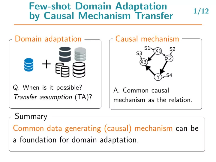
Few-shot Domain Adaptation 1/12 by Causal Mechanism Transfer Domain adaptation Causal mechanism Q. When is it possible? A. Common causal Transfer assumption (TA)? mechanism as the relation. Summary Common data generating (causal) mechanism can be a foundation for domain adaptation.

What’s the intuition? 2/12 Intuition Humans care about finding causal knowledge be- cause, once discovered, it applies to different systems. Motivating example: Regional disease prediction • Predict disease risk from medical records. [1] • Data distributions may vary for different lifestyles. • Common pathological mechanism across regions.

Few-shot Domain Adaptation by Causal Mechanism Transfer Takeshi Teshima 12 , Issei Sato 12 , and Masashi Sugiyama 21 1 The University of Tokyo 2 RIKEN (This work was supported by RIKEN Junior Research Associate Program.)

Preliminary: Causal model (SEMs) 3/12 Structural Equation Models (SEMs) 1, 2 [2] • Generative model for the joint distribution of data. • Consists of deterministic functions of the form:  X 1 = f ′ 1 (pa 1 , S 1 )      = f ′ 2 (pa 2 , S 2 ) X 2  = f ′ 3 (pa 3 , S 3 ) X 3      Y = f ′ 4 (pa 4 , S 4 )  and an independent distribution of ( S 1 , . . . , S D ) . 1 More precisely, NPSEM-IE (Nonparametric SEM with Independent Errors). 2 Acyclicity is assumed.

Nonlinear-ICA and reduced-form SEM 4/12 Reduced form: Structural equations solved for ( X , Y ) .  X 1 = f ′ 1 (pa 1 , S 1 )       X 1 S 1         = f ′ 2 (pa 2 , S 2 ) ⇒  X 2 X 2 S 2      = f         X 3 S 3 X 3 = f ′ 3 (pa 3 , S 3 )              Y S 4  = f ′ 4 (pa 4 , S 4 )  Y  Structural equations Reduced form • Under certain identification conditions , nonlinear-ICA 3 methods can estimate f (we use it in our method). 3 ICA = Independent component analysis.

Formulation 1/3: Data and goal 5/12 Basic setup: regression domain adaptation 1. Homogeneous (i.e., all domains in the same space) X × Y ⊂ R D − 1 × R 2. Multi-source (i.e., multiple source domains) nk i.i.d. D k = { ( x k,i , y k,i ) } ∼ p src( k ) ( k = 1 , . . . , K ) (large n k ) i =1 3. Few-shot supervised (i.e., target data with labels) i.i.d. { ( x tar ,i , y tar ,i ) } n tar ∼ p tar ( n tar is small) i =1 Goal: accurate predictor for the target distribution Find g : R D − 1 → R s.t. R ( g ) := E tar ℓ ( g, X, Y ) is minimal. ( ℓ : loss function)

Formulation 2/3: Each domain 6/12 • Each domain follows a nonlinear-ICA model. Dist. p consists of ( f, q ) 1. D -dimensional ICs S are sampled from q . 2. Invertible f transforms S into ( X, Y ) = f ( S ) . • f can be estimated by ICA under assumptions. • f corresponds to the reduced form of an SEM.

Formulation 3/3: Key assumption 7/12 • Key Assumption: generative mechanism f is common. • Allow flexible shift in q ⇝ Enables DA among seemingly very different distributions.

Proposed method: Strategy 8/12 f − 1 ˆ ˆ f → → → Idea: How to exploit the assumption 1. Estimate f using source domain data (NLICA). 2. Estimate ICs of the target data using ˆ f − 1 . 3. Reshuffle the independent components. 4. Generate target data from reshuffled ICs using ˆ f . 5. Train the predictor g on the generated data.

Theoretical analyses 9/12 Q1. How does the method statistically help? Theorem: If ˆ f = f , the proposed risk estimator is the uniformly minimum variance unbiased risk estimator. The method should help in terms of variance. Q2. What happens when ˆ f ̸ = f ? What’s the catch? Theorem: generalization error bound for ˆ f ̸ = f . Mitigate overfitting. Introduce bias.

Experiment: Setup 10/12 • Dataset: Gasoline consumption dataset [3] . ▶ Panel data from econometrics (SEMs have been applied). ▶ 18 countries (=domains), 19 years, D = 4 . • Baselines for regression domain adaptation. Name Compared method (predictor: KRR) TarOnly Train on target. SrcOnly Train on source. S&TV Train on source, CV on target. TrAdaBoost Boosting for few-shot regression transfer [4] . IW Joint importance weight using RuLSIF [5] . GDM Generalized discrepancy minimization [6] . Copula Non-parametric R-vine copula method [7] . LOO (reference) LOOCV error estimate.

Experiment: Result 11/12 Target (LOO) TrgOnly Prop SrcOnly S&TV TrAda GDM Copula IW(.0) IW(.5) IW(.95) AUT 1 5.88 5.39 9.67 9.84 5.78 31.56 27.33 39.72 39.45 39.18 (1.60) (1.86) (0.57) (0.62) (2.15) (1.39) (0.77) (0.74) (0.72) (0.76) BEL 1 10.70 7.94 8.19 9.48 8.10 89.10 119.86 105.15 105.28 104.30 (7.50) (2.19) (0.68) (0.91) (1.88) (4.12) (2.64) (2.96) (2.95) (2.95) CAN 1 5.16 3.84 157.74 156.65 51.94 516.90 406.91 592.21 591.21 589.87 (1.36) (0.98) (8.83) (10.69) (30.06) (4.45) (1.59) (1.87) (1.84) (1.91) DNK 1 3.26 3.23 30.79 28.12 25.60 16.84 14.46 22.15 22.11 21.72 (0.61) (0.63) (0.93) (1.67) (13.11) (0.85) (0.79) (1.10) (1.10) (1.07) FRA 1 2.79 1.92 4.67 3.05 52.65 91.69 156.29 116.32 116.54 115.29 (1.10) (0.66) (0.41) (0.11) (25.83) (1.34) (1.96) (1.27) (1.25) (1.28) DEU 1 16.99 6.71 229.65 210.59 341.03 739.29 929.03 817.50 818.13 812.60 (8.04) (1.23) (9.13) (14.99) (157.80) (11.81) (4.85) (4.60) (4.55) (4.57) GRC 1 3.80 3.55 5.30 5.75 11.78 26.90 23.05 47.07 45.50 45.72 (2.21) (1.79) (0.90) (0.68) (2.36) (1.89) (0.53) (1.92) (1.82) (2.00) IRL 1 3.05 4.35 135.57 12.34 23.40 3.84 26.60 6.38 6.31 6.16 (0.34) (1.25) (5.64) (0.58) (17.50) (0.22) (0.59) (0.13) (0.14) (0.13) ITA 1 13.00 14.05 35.29 39.27 87.34 226.95 343.10 244.25 244.84 242.60 (4.15) (4.81) (1.83) (2.52) (24.05) (11.14) (10.04) (8.50) (8.58) (8.46) JPN 1 10.55 12.32 8.10 8.38 18.81 95.58 71.02 135.24 134.89 134.16 (4.67) (4.95) (1.05) (1.07) (4.59) (7.89) (5.08) (13.57) (13.50) (13.43) NLD 1 3.75 3.87 0.99 0.99 9.45 28.35 29.53 33.28 33.23 33.14 (0.80) (0.79) (0.06) (0.05) (1.43) (1.62) (1.58) (1.78) (1.77) (1.77) NOR 1 2.70 2.82 1.86 1.63 24.25 23.36 31.37 27.86 27.86 27.52 (0.51) (0.73) (0.29) (0.11) (12.50) (0.88) (1.17) (0.94) (0.93) (0.91) ESP 1 5.18 6.09 5.17 4.29 14.85 33.16 152.59 53.53 52.56 52.06 Proposed > TrgOnly when the other methods using (1.05) (1.53) (1.14) (0.72) (4.20) (6.99) (6.19) (2.47) (2.42) (2.40) SWE 1 6.44 5.47 2.48 2.02 2.18 15.53 2706.85 118.46 118.23 118.27 (2.66) (2.63) (0.23) (0.21) (0.25) (2.59) (17.91) (1.64) (1.64) (1.64) CHE 1 3.51 2.90 43.59 7.48 38.32 8.43 29.71 9.72 9.71 9.79 source domain data suffer from negative transfer. (0.46) (0.37) (1.77) (0.49) (9.03) (0.24) (0.53) (0.29) (0.29) (0.28) TUR 1 1.65 1.06 1.22 0.91 2.19 64.26 142.84 159.79 157.89 157.13 (0.47) (0.15) (0.18) (0.09) (0.34) (5.71) (2.04) (2.63) (2.63) (2.69) GBR 1 5.95 2.66 15.92 10.05 7.57 50.04 68.70 70.98 70.87 69.72 (1.86) (0.57) (1.02) (1.47) (5.10) (1.75) (1.25) (1.01) (0.99) (1.01) USA 1 4.98 1.60 21.53 12.28 2.06 308.69 244.90 462.51 464.75 465.88 (1.96) (0.42) (3.30) (2.52) (0.47) (5.20) (1.82) (2.14) (2.08) (2.16) #Best - 2 10 2 4 0 0 0 0 0 0

Take-home message 12/12 1. Transfer assumption of shared generative mechanism. Developed a few-shot regression DA method. 2. Proposed method extracts and uses the causal model to reduce overfitting via data augmentation. 3. Experiment with real-world data demonstrate the validity. f − 1 ˆ ˆ f → → →

References [1] P. Yadav, M. Steinbach, V. Kumar, and G. Simon, ‘Mining electronic health records (EHRs): A survey’, ACM Computing Surveys , vol. 50, no. 6, pp. 1–40, 2018. [2] J. Pearl, Causality: Models, Reasoning and Inference , Second. Cambridge, U.K. ; New York: Cambridge University Press, 2009. [3] W. H. Greene, Econometric Analysis , Seventh. Boston: Prentice Hall, 2012. [4] D. Pardoe and P. Stone, ‘Boosting for regression transfer’, in Proceedings of the Twenty-Seventh International Conference on Machine Learning , Haifa, Israel, 2010, pp. 863–870. [5] M. Yamada, T. Suzuki, T. Kanamori, H. Hachiya, and M. Sugiyama, ‘Relative density-ratio estimation for robust distribution comparison’, in Advances in Neural Information Processing Systems 24 , J. Shawe-Taylor, R. S. Zemel, P. L. Bartlett, F. Pereira, and K. Q. Weinberger, Eds., Curran Associates, Inc., 2011, pp. 594–602. [6] C. Cortes, M. Mohri, and A. M. Medina, ‘Adaptation based on generalized discrepancy’, Journal of Machine Learning Research , vol. 20, no. 1, pp. 1–30, 2019.

References (cont.) [7] D. Lopez-paz, J. M. Hernndez-lobato, and B. Schlkopf, ‘Semi-supervised domain adaptation with non-parametric copulas’, in Advances in Neural Information Processing Systems 25 , F. Pereira, C. J. C. Burges, L. Bottou, and K. Q. Weinberger, Eds., Curran Associates, Inc., 2012, pp. 665–673.