ICMMES Conference, Hong Kong, July 25-29, 2005 On Direct and Adjoint Lattice Boltzmann Equations Fran¸ cois Dubois Numerical Analysis and Partial Differential Equations Department of Mathematics, Universit´ e Paris Sud conjoint work with Mahmed Bouzidi, Pierre Lallemand, Mahdi Tekitek Edition du 27 septembre 2005.
On Direct and Adjoint Lattice Boltzmann Equations Scope of the lecture 1) On Taylor and Chapman Enskog expansions for discrete Boltzmann dynamics 2) Inverse methodology for a linear thermal problem 3) Adjoint Lattice Boltzmann Equation ICMMES Conference, Hong Kong, July 28, 2005
General framework x : a node of the lattice ∆ t : the (small) time step components v α v j : discrete celerity in the lattice, j , α = 1 , 2 then x + v j ∆ t is an other node of the lattice f j ( x , t ) : density of particles having the velocity v j at node x and at discrete time t . � m 0 = ρ ≡ f j : density of matter j � m α = q α ≡ j f j : component number α of the momentum v α j W ≡ ( ρ , q 1 , q 2 ) : conserved variables ICMMES Conference, Hong Kong, July 28, 2005
General framework 2 5 6 3 1 0 7 8 4 Neighbourhood of a vertex x for the D2Q9 LBE model ICMMES Conference, Hong Kong, July 28, 2005
d’Humi` eres (1992) representation of the discrete dynamics � m k ≡ j f j ( k ≥ 3) : other components of the momentum M k j remark that we have M 0 j = 1 and M α j = v α j m k eq and f j eq : equilibrium momenta and velocity distribution • collision step ∗ ≡ m i ≡ m i m i eq : conserved momenta ( i = 0 , 1 , 2) during the collision ∗ = (1 − s k ) m k + s k m k m k k ≥ 3 : nonconserved momenta eq , Classical stability condition for the explicit Euler scheme : 0 < s k < 2 � ( M − 1 ) j f j k m k ∗ ≡ ∗ : particle distribution after the collision k • advection step f j ( x , t + ∆ t ) = f j ∗ ( x − v j ∆ t , t ) ICMMES Conference, Hong Kong, July 28, 2005
Taylor expansion at the order zero f j ( x , t + ∆ t ) ≡ f j ∗ ( x − v j ∆ t , t ) f j ( x , t + ∆ t ) = f j ( x , t ) + O(∆ t ) f j ∗ ( x − v j ∆ t , t ) = f j ∗ ( x , t ) + O(∆ t ) � ∗ = m k + O(∆ t ) m k M k j f j then ∗ = j ∗ − m k = O(∆ t ) m k ∗ − m k ≡ − s k ( m k − m k m k but eq ) and s k > 0 if k ≥ 3 m k = m k thus eq + O(∆ t ) m k ∗ = m k eq + O(∆ t ) coming back in the space of velocity distribution : f j = f j eq + O(∆ t ) f j ∗ = f j eq + O(∆ t ) . ICMMES Conference, Hong Kong, July 28, 2005
Taylor expansion at the first order f j ( x , t + ∆ t ) ≡ f j ∗ ( x − v j ∆ t , t ) = f j ( x , t ) + ∆ t ∂ t f j + O(∆ t 2 ) f j ( x , t + ∆ t ) ∗ ( x , t ) − ∆ t v β ∗ + O(∆ t 2 ) f j ∗ ( x − v j ∆ t , t ) = f j j ∂ β f j we take the moment of order k of this identity � m k + ∆ t ∂ t m k + O(∆ t 2 ) = m k j v β M k j ∂ β f j ∗ + O(∆ t 2 ) ∗ − ∆ t j we use the previous Taylor expansion at the order zero � m k + ∆ t ∂ t m k j v β eq + O(∆ t 2 ) = m k M k j ∂ β f j eq + O(∆ t 2 ) ∗ − ∆ t j ∂ t ρ + ∂ β q β = O(∆ t ) • k = 0 : conservation of mass � F α β ≡ j v β v α j f j introduce the tensor eq j ∂ t q α + ∂ β F α β = O(∆ t ) • k = α : conservation of impulsion ICMMES Conference, Hong Kong, July 28, 2005
Taylor expansion at the first order � m k + ∆ t ∂ t m k j v β eq + O(∆ t 2 ) = m k M k j ∂ β f j eq + O(∆ t 2 ) ∗ − ∆ t j m k − m k ∗ ≡ s k ( m k − m k but eq ) if k ≥ 3 � � introduce θ k = ∂ t m k j v β eq + v β M k j ∂ β f j M k j ( ∂ t f j j ∂ β f j eq + eq ≡ eq ) j j θ i = O(∆ t ) : for i = 0 , 1 , 2 , Euler equations of gas dynamics eq − ∆ t m k = m k θ k + O(∆ t 2 ) then for k ≥ 3 : s k � 1 � ∆ t θ k + O(∆ t 2 ) m k ∗ = m k eq − − 1 s k � 1 � � k ∂ β θ k + O(∆ t 2 ) ( M − 1 ) j ∂ β f j ∗ = ∂ β f j eq − ∆ t − 1 s k k ≥ 3 ICMMES Conference, Hong Kong, July 28, 2005
Taylor expansion at the second order f j ( x , t + ∆ t ) ≡ f j ∗ ( x − v j ∆ t , t ) = f j ( x , t ) + ∆ t ∂ t f j + 1 2 ∆ t 2 ∂ 2 tt f j + O(∆ t 3 ) f j ( x , t + ∆ t ) 2 ∆ t 2 v β f j ∗ ( x − v j ∆ t , t ) = f j ∗ ( x , t ) − ∆ t v β j ∂ β f j j v γ βγ f j ∗ + 1 j ∂ 2 ∗ + O(∆ t 3 ) we take the moment of order i (0 ≤ i ≤ 2) of this identity m i + ∆ t ∂ t m i + 1 tt m i + O(∆ t 3 ) = 2 ∆ t 2 ∂ 2 � 2 ∆ t 2 � ∗ + 1 j v β j v β j v γ j ∂ 2 ∗ + O(∆ t 3 ) = m i M i j ∂ β f j M i βγ f j ∗ − ∆ t j j we use the microscopic conservation m i ∗ = m i and the previous Taylor expansion at the order one : � ∂ t m i + 1 tt m i + O(∆ t 2 ) = − 2 ∆ t ∂ 2 j v β M i j ∂ β f j eq + j � 1 � � � k ∂ β θ k + 1 j v β ( M − 1 ) j j v β j v γ M i M i j ∂ 2 βγ f j eq + O(∆ t 2 ) + ∆ t − 1 2 ∆ t j s k j, k ≥ 3 j ICMMES Conference, Hong Kong, July 28, 2005
Taylor expansion at the second order � 1 � � � ∂ t m i + k ∂ β θ k + j v β j v β ( M − 1 ) j M i j ∂ β f j M i eq = ∆ t − 1 j s k j j, k ≥ 3 � � � + ∆ t tt m i + j v β j v γ − ∂ 2 j ∂ 2 + O(∆ t 2 ) M i βγ f j eq 2 j • i = 0 : conservation of mass M 0 j ≡ 1 and the first sum is null � tβ q β = − ∂ β ∂ t q β = ∂ 2 βγ F β γ = ∂ 2 tt ρ = − ∂ 2 v β j v γ j ∂ 2 βγ f j eq j ∂ t ρ + ∂ β q β = O(∆ t 2 ) and the second sum is null. Then • i = α : conservation of impulsion � 1 � � � � � � ∂ t q α + ∂ β θ k + j v β j v β j ( M − 1 ) j v α j ∂ β f j v α eq = ∆ t − 1 k s k j k ≥ 3 j � � � + ∆ t tt q α + j v β j v γ − ∂ 2 j ∂ 2 + O(∆ t 2 ) v α βγ f j eq 2 j ICMMES Conference, Hong Kong, July 28, 2005
From Taylor to Chapman-Enskog � � tt q α + eq = ∂ t ∂ β F α β + j v β j v γ j v β j v γ − ∂ 2 j ∂ 2 j ∂ 2 v α βγ f j v α βγ f j eq j j � � � j v β eq + v γ v α ∂ t f j j ∂ γ f j = ∂ β eq j j � � j v β ( M − 1 ) j v α k θ k = ∂ β j j k � � � � θ k + O(∆ t ) j v β j ( M − 1 ) j v α = ∂ β k k ≥ 3 j � Λ α β j v β j ( M − 1 ) j v α introduce the tensor ≡ k k j � 1 � � � ∂ β θ k + ∆ t ∂ t q α + ∂ β F α β = ∆ t Λ α β Λ α β ∂ β θ k − 1 k k s k 2 k ≥ 3 k ≥ 3 � 1 � � − 1 ∂ t q α + ∂ β F α β − ∆ t ∂ β θ k = O(∆ t 2 ) : Chapman-Enskog ! Λ α β k 2 s k k ≥ 3 ICMMES Conference, Hong Kong, July 28, 2005
Unidimensional heat equation with the D2Q9 LBE model periodic boundary conditions for the y direction equilibrium velocity = 0 equilibrium energy = − 2 density equilibrium (energy) 2 = density ∗ = v x + s 1 (0 − v x ) v x relaxation of velocities : � 1 � κ = 1 − 1 3 s 1 2 s energy = 1 s (energy) 2 = 1 s fluxofenergy = 1 , 2 s XX = s XY = 1 , 4 ICMMES Conference, Hong Kong, July 28, 2005
Inverse methodology for a linear thermal problem � � ∂u ∂t − ∂ κ∂u = 0 , 0 ≤ x ≤ L , t > 0 ∂x ∂x ∂u ∂n ( x = 0 , t ) = Φ( t ) , t > 0 ∂u ∂n ( x = L , t ) = 0 , t > 0 u ( x , t = 0) = 0 , 0 ≤ x ≤ L unknown flux function Φ( t ) observed values ψ ( x k , t ) ≈ u ( x k , t ) � � Inverse problem : does exists a function ψ ( x k , • ) k �− → Φ( • ) ? T � � J (Φ) = 1 | u ( x k , t ) − ψ ( x k , t ) | 2 “cost” error functional : 2 t =0 k observed ICMMES Conference, Hong Kong, July 28, 2005
Inverse methodology for a linear thermal problem use the linearity of the problem ! Elementary discrete solution : θ ( j ∆ x , n ∆ t ) ≡ θ j ( n ∆ t ) � � ∂θ ∂t − ∂ κ ∂θ = 0 , 0 ≤ x ≤ L , t > 0 ∂x ∂x ∂θ ∂n ( x = 0 , t = 1) = 1 , 0 < t < ∆ t ∂θ ∂n ( x = 0 , t ) = 0 , t > ∆ t ∂θ ∂n ( x = L , t ) = 0 , t > 0 θ ( x , t = 0) = 0 , 0 ≤ x ≤ L then N N � � Φ( t ) = ϕ n δ ( t − n ∆ t ) and u ( j ∆ x , t ) = ϕ n θ j ( t − n ∆ t ) . n =1 n =1 ICMMES Conference, Hong Kong, July 28, 2005
Inverse methodology for a linear thermal problem Data for Bouzidi experiment ∆ x = 1 ∆ t = 1 0 ≤ x ≤ L = 110 0 ≤ t ≤ T = 500 Φ( t ) ≡ 0 if t ≥ N = 70 observation points : k = 10 , 20 , 30 , 40 , 50 ICMMES Conference, Hong Kong, July 28, 2005
Inverse methodology for a linear thermal problem initial time time=50 0.7 time=100 time=150 time=200 0.6 time=250 time=300 time=350 time=400 0.5 time=450 0.4 0.3 0.2 0.1 0 0 20 40 60 80 100 grid number Elementary temperature θ j ( n ∆ t ) for a unity flux ICMMES Conference, Hong Kong, July 28, 2005
Inverse methodology for a linear thermal problem initial time time=50 time=100 0.1 time=150 time=200 time=250 time=300 time=350 0.08 time=400 time=450 0.06 0.04 0.02 0 2 4 6 8 10 12 14 grid number (zoom near the left boundary) Elementary temperature θ j ( n ∆ t ) for a unity flux ICMMES Conference, Hong Kong, July 28, 2005
Recommend
More recommend
Unleash a World of Digital Possibilities—Browse, Share, and Explore Content Without Boundaries