Ocean mesoscale eddies, air-sea interactions and regional climate: - PowerPoint PPT Presentation

Ocean mesoscale eddies, air-sea interactions and regional climate: regional coupled climate modeling Hyodae Seo Woods Hole Oceanographic Institution APEC Climate Center, Busan, Korea September 13, 2013

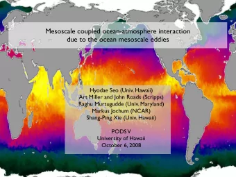
Sea Ice Margin North Atlantic Current Oyashio Sub-polar Front K-O Extension Coastal Gulf Stream Upwelling Kuroshio Loop Current Upwelling Tropical Instability Waves TIW Equatorial Cold Tongue Coastal Coastal Upwelling Upwelling Antarctic Circumpolar Current Global SST from AMSR-E on June 1, 2003 http://aqua.nasa.gov/highlight.php

Air-sea interactions on different oceanic scales Oceanic basin-scale: NAO Oceanic mesoscale: eddies Correlation in wind speed and SST Spatially high-passed wind, SST Positive correlation (Warm SST ➔ Stronger wind) Xie et al. 2004 Stronger wind ➔ colder SST (Negative correlation). Kushnir et al. 2002

Mechanisms for positive correlation between SST and wind speed PBL Height QSCAT WIND STRESS TRMM SST Cold Warm TIWs trigger mesoscale response in the atmospheric boundary layer. Limited information from satellite and in situ F IG . 9. (top) Longitude–height section of zonal wind velocity (vectors) and virtual potential temperature (K)(contours Hashizume et al. 2002 data makes fuller understanding of dynamics of fine-scale interactions difficult. Destabilized ABL over warm SST ➔ Downward momentum mixing ➔ Need a coupled model with improved ➔ Accelerating surface winds representation of oceanic eddies AND their (Wallace et al. 1998) influence on the atmosphere.

Scripps Coupled Ocean-Atmosphere Regional (SCOAR) Model SCOAR Model Atmosphere Ocean • Study mesoscale Atmospheric Forcing 1. Weather Research 1. Regional Ocean ocean-atmosphere and Forecasting Model Modeling System interactions and large- (WRF) (ROMS) scale climate. Flux-SST Coupler • An input-output-based 2. Process Study 2. Scripps coupler and sequential Ocean Model Regional Spectral (PSOM) Model (RSM) coupling. SST, Current • Great portability and applicability Lateral Boundary Conditions: IPCC models, reanalyses Seo, Miller and Roads, J. Climate 2007

Overview of my talk • Regional Coupled Model 1.Dynamics of coherent variations in the atmosphere to SST (1)TIWs in the equatorial Pacific and Atlantic (2) Sea ice in the Arctic Ocean 2. Role of ocean dynamics in shaping SST warming in a changing climate in the equatorial Atlantic • Summary and discussion

Mesoscale Air-Sea Interactions over tropical instability waves

How do these wind responses feedback to ocean mesoscale variability? Combined EOF 1 of SST & Wind vectors ➀ Direct influence from SST: SST ➜ 훕′ ② Modification of wind stress curl/div � � SST ➜ � · 훕′ � � SST ➜ �� 훕′ Feedback to TIWs through ➀         BT BC     U ⋅ K e + $ u ⋅ K ∇ ⋅ ( $ u $ p ) − g $ ρ $ w + ρ o ( − $ u ⋅ ( $ u ⋅ U )) ∇ ∇ e = − ∇  sfc ⋅      2 $ u + " " + ρ o A h $ u ⋅ ∇ u + ρ o $ u ⋅ ( A v $ u z ) z τ z

Anomalies in current and wind stress are opposite in direction, meaning wind response damping the ocean! Correlation of v ′ sfc and 훕 y ′ Eddy kinetic energy budget Atlantic TIWs Barotropic Wind energy input conversion 4N Latitude v sfc τ y τ y’ • Wind contribution to TIWs is ~10% of Mean BT conversion rate. EQ • A small but significant damping of TIW. • Wind and current are negatively correlated. • Wind-current coupling ➔ energy sink

② Modification of wind stress curl by SST gradients:

WARM Coherent variability of wind stress curl and divergence to SST gradients! DIV CURL OBS MODEL COLD SST EQ Curl EQ Divergence EQ

1 Is this eddy-mediated Ekman pumping important r w f r � T w ¼ for ocean circulation? Yes! EK PDF of W EK by mean and perturbation 50E − 60E, 6N − 12.5N averages JJAS 1995 − 2006 •Eddy-induced Ekman pumping 10 vertical velocity exhibit a 9 comparable dynamic range to that 8 by mean Ekman pumping. Mean Wek 7 Anomaly Percentage of OBS Wek’ 6 • This W EK ’ is additional wind 5 stress curl forcing of the ocean. 4 3 •This effect will influence the mean 2 state through low-frequency 1 rectification. 0 − 3 − 2 − 1 0 1 2 3 Ekman pumping velocity, meter day − 1

A similar story is applied to the ABL fields in the Arctic over sea ice: Separation of spatial scale of wind response

Polar WRF simulation Polar WRF domain, in situ datasets overlaid • Polar WRF: Hines and Bromwich with STD of SON SIC (2008) • WRF optimized for polar regions • Modified surface layer model for improved surface energy balance • Experiments • November 2008 - October 2009 • Sea ice forcing: • NT: NASA Team Algorithm • BT: NASA Bootstrap Algorithm

NT NT-BT Pan-Arctic response pattern Focusing on NT - BT in September 2009 Large change in ABL compared to the mean values East Siberian Sea Mean Difference T2 -5 °C +5 °C PBLH 450 m 100 m TCWP 60 gm -2 10 gm -2 SIC uncertainty is a decisive factor for hindcast skill! • SIC difference and ABL sensitivity on the total cloud water path comparable basin-scales

Arctic-basin averaged vertical profiles difference (NT -BT) • ABL stability adjustment to SST: Wallace et al., (1989). • Less SIC ➔ Higher PBL • The basin-wide increase in air temperatures below PBL. ➜ 58-m increase in PBLH

Arctic-basin averaged vertical profiles difference (NT -BT) • ABL stability adjustment to SST: Wallace et al., (1989). • Less SIC ➔ Higher PBL • The basin-wide increase in air temperatures below PBL. • Increased cloud water path near the top of PBL. ➜ 58-m increase in PBLH

Arctic-basin averaged vertical profiles difference (NT -BT) • ABL stability adjustment to SST: Wallace et al., (1989). • Less SIC ➔ Higher PBL • The basin-wide increase in air temperatures below PBL. • Increased cloud water path near the top of PBL. • Stronger wind below 100 meter but weaker wind aloft • Reminiscent of what is happening in mid to low latitudes! ➜ 58-m increase in PBLH F . 9. (top) Longitude–height section of zonal wind velocity (vectors) and virtual potential temperature (K) (contours Observations of ABL evolution in the eastern tropical Pacific Hashizume et al. (2002)

Contrasting responses in two near-surface wind fields: W10 and Wg ( ≈∇ SLP) NT - BT in September 2009 W10 NT Mean W10 NT -BT • Stronger W10 with reduced SIC • Most dramatic changes in the interior Arctic • >10% change of the mean. Wg NT Mean Wg NT -BT • Reduced Wg along the ice margins! • Significant changes compared to the mean Wg • No significant changes in the interior Arctic.

Wg response is more pronounced on the smaller scale than W10 • A simple marine boundary layer model of Lindzen and Nigam (1987): • Assuming s teady flow, no advection, linear friction, ρ o ∇⋅  ε 2 + f 2 ( ) ε ( ) ) = − ∇ 2 P ( u • Div. /Conv. of surface wind is linearly proportional to SIC-induced Laplacian of SLP • � 2 would be effective in highlighting small-scale response, e.g., along the sea ice margins.

What is the role of ocean dynamics in shaping regional SST pattern in a warming climate? The Equatorial Atlantic Ocean.. • IPCC-class models have large biases in simulation of the equatorial climate - Especially in the Atlantic. - A reversed east-west gradient. - Underestimation of equatorial currents, upwelling and TIWs. Richter and Xie 2008 obs CMIP3 models a SST OBS CMIP SCOAR longitudes on equator b

Model and experiments CTL • CTL : RSM (NCEP2 6hrly) + ROMS (SODA ➜ ➜ ATM monthly) ROMS RSM ➜ ➜ SST • 25 km ROMS + 50 km RSM ➜ ➜ • 28-yr. integration: 1980-2007 NCEP2 SODA • CO2=348 PPM GW • δ =GFDL CM2.1 monthly difference: ➜ ➜ Flux (2045-2050: A1B)-(1996-2000: 20C); 10- ROMS RSM ➜ ➜ member ensemble mean SST ➜ ➜ • GW : RSM (NCEP2 6-hrly+ δ ) + ROMS (SODA NCEP2+ δ SODA+ δ monthly+ δ ) • CO2=521.75 PPM pseudo-global warming method in a regional coupled model (Seo and Xie 2011)

Change in annual mean state (GW-CTL) SST, Wind Precip, net heat flux • Different equatorial ocean response: - Reduced warming (more upwelling) in the equator. CM2.1 - Cross-equatorial southerly wind is stronger on equator. • Similar large-scale atmospheric response - Increased (decreased) SCOAR rainfall in the tropical northeast (south) Atlantic.

Response of ocean to the cross-equatorial southerly wind? 1. Reduced warming on the equator? 2. Change in equatorial currents?

1. Reduced warming in the cold tongue is due to the increased upwelling. under global warming ➀ ➁ ➂ ➃ x=<x>+x * <>: present-day mean (CTL) ! *: Perturbation (GW-CTL) ➁ ➁ Radiative heating ➜ dT * /dZ >0 : Ocean Dynamical Thermostat (in the Pacific: Clement et al. 1996, Cane et al. 1997) ➂ ➂ Cross-equatorial wind ➜ w * >0. ✔ Atlantic ( w * , ➂ ) vs Pacific ( dT * /dZ, ➁ )

2. Stronger upwelling associated with stronger Equatorial Undercurrent SCOAR U SODA (OBS) U CM2.1 U NECC sSEC nSEC EUC Depth [m] [cm] Latitude • Weak EUC and weak upwelling in CM2.1. • Strong EUC and strong upwelling in SCOAR. • Stronger currents have an important implication for the dynamic instability. 30°W-10°W, 1998-2007