Object Detection EECS 442 Prof. David Fouhey Winter 2019, - PowerPoint PPT Presentation

Object Detection EECS 442 – Prof. David Fouhey Winter 2019, University of Michigan http://web.eecs.umich.edu/~fouhey/teaching/EECS442_W19/

Last Time “Semantic Segmentation”: Label each pixel with the object category it belongs to. Input Target CNN

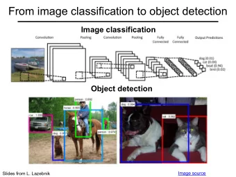
Today – Object Detection “Object Detection”: Draw a box around each instance of a list of categories Input Target CNN

The Wrong Way To Do It 1 F CNN 1 Starting point: Can predict the probability of F classes P(cat), P(goose), … P(tractor)

The Wrong Way To Do It 1 F 1 CNN 4 1 1 Add another output (why not): Predict the bounding box of the object [x,y,width,height] or [minX,minY,maxX,maxY]

The Wrong Way To Do It 1 F Lc 1 CNN 4 1 Lb 1 Put a loss on it: Penalize mistakes on the classes with Lc = negative log-likelihood Lb = L2 loss

The Wrong Way To Do It 1 F Lc 1 CNN L + 4 1 Lb 1 Add losses, backpropagate Final loss: L = Lc + λ Lb Why do we need the λ ?

The Wrong Way To Do It 1 F Lc 1 CNN L + 4 1 Lb 1 Now there are two ducks. How many outputs do we need? F, 4, F, 4 = 2*(F+4)

The Wrong Way To Do It 1 F Lc 1 CNN L + 4 1 Lb 1 Now it’s a herd of cows. We need lots of outputs (in fact the precise number of objects that are in the image, which is circular reasoning).

In General • Usually can’t do varying -size outputs. • Even if we could, think about how you would solve it if you were a network. Bottleneck has to encode where the objects are for all objects and all N FN 1 1 4N 1 1

An Alternate Approach Examine every sub-window and determine if it is a tight box around an object Yes No? Hold this thought No

Sliding Window Classification Let’s assume we’re looking for pedestrians in a box with a fixed aspect ratio. Slide credit: J. Hays

Sliding Window Key idea – just try all the subwindows in the image at all positions. Slide credit: J. Hays

Generating hypotheses Key idea – just try all the subwindows in the image at all positions and scales. Note – Template did not change size Slide credit: J. Hays

Each window classified separately Slide credit: J. Hays

How Many Boxes Are There? Given a HxW image and a “template” by of size by, bx. Q. How many sub-boxes are there of size (by,bx)? bx A. (H-by)*(W-bx) This is before considering adding: • scales (by*s,bx*s) • aspect ratios (by*sy,bx*sx)

Challenges of Object Detection • Have to evaluate tons of boxes • Positive instances of objects are extremely rare How many ways can we get the box wrong? 1. Wrong left x 2. Wrong right x 3. Wrong top y 4. Wrong bottom y

Prime-time TV Are You Smarter Than A 5 th Grader? Adults compete with 5 th graders on elementary school facts. Adults often not smarter.

Computer Vision TV Are You Smarter Than A Random Number Generator? Models trained on data compete with making random guesses. Models often not better.

Are You Smarter than a Random Number Generator? • Prob. of guessing 1k-way classification? • 1/1,000 • Prob. of guessing all 4 bounding box corners within 10% of image size ? • (1/10)*(1/10)*(1/10)*(1/10)=1/10,000 • Probability of guessing both: 1/10,000,000 • Detection is hard (via guessing and in general) • Should always compare against guessing or picking most likely output label

Evaluating – Bounding Boxes Raise your hand when you think the detection stops being correct.

Evaluating – Bounding Boxes Standard metric for two boxes: Intersection over union/IoU/Jaccard coefficient / Jaccard example credit: P. Kraehenbuehl et al. ECCV 2014

Evaluating Performance • Remember: accuracy = average of whether prediction is correct • Suppose I have a system that gets 99% accuracy in person detection. • What’s wrong? • I can get that by just saying no object everywhere!

Evaluating Performance • True detection: high intersection over union • Precision: #true detections / #detections • Recall: #true detections / #true positives Reject everything: no mistakes 1 Ideal! Precision Summarize by area under curve (avg. precision) Accept everything: 0 Miss nothing Recall 1

Generic object detection Slide Credit: S. Lazebnik

Histograms of oriented gradients (HOG) Partition image into blocks and compute histogram of gradient orientations in each block HxWx3 Image H’xW’xC’ Image Image credit: N. Snavely N. Dalal and B. Triggs, Histograms of Oriented Gradients for Human Detection, CVPR 2005 Slide Credit: S. Lazebnik

Pedestrian detection with HOG • Train a pedestrian template using a linear support vector machine positive training examples negative training examples N. Dalal and B. Triggs, Histograms of Oriented Gradients for Human Detection, CVPR 2005 Slide Credit: S. Lazebnik

Pedestrian detection with HOG • Train pedestrian “template” using a linear svm • At test time, convolve feature map with template • Find local maxima of response • For multi-scale detection, repeat over multiple levels of a HOG pyramid HOG feature map Detector response map Template N. Dalal and B. Triggs, Histograms of Oriented Gradients for Human Detection, CVPR 2005 Slide Credit: S. Lazebnik

Example detections [Dalal and Triggs, CVPR 2005] Slide Credit: S. Lazebnik

PASCAL VOC Challenge (2005-2012) • 20 challenge classes: • Person • Animals: bird, cat, cow, dog, horse, sheep • Vehicles: aeroplane, bicycle, boat, bus, car, motorbike, train • Indoor: bottle, chair, dining table, potted plant, sofa, tv/monitor • Dataset size (by 2012): 11.5K training/validation images, 27K bounding boxes, 7K segmentations http://host.robots.ox.ac.uk/pascal/VOC/ Slide Credit: S. Lazebnik

Object detection progress PASCAL VOC Before CNNs Using CNNs Source: R. Girshick

Region Proposals Do I need to spend a lot of time filtering all the boxes covering grass?

Region proposals • As an alternative to sliding window search, evaluate a few hundred region proposals • Can use slower but more powerful features and classifiers • Proposal mechanism can be category-independent • Proposal mechanism can be trained Slide Credit: S. Lazebnik

R-CNN: Region proposals + CNN features Source: R. Girshick Classify regions with SVMs SVMs SVMs SVMs Forward each region through ConvNet ConvNet ConvNet ConvNet Warped image regions Region proposals Input image R. Girshick, J. Donahue, T. Darrell, and J. Malik, Rich Feature Hierarchies for Accurate Object Detection and Semantic Segmentation, CVPR 2014.

R-CNN details • Regions : ~2000 Selective Search proposals • Network : AlexNet pre-trained on ImageNet (1000 classes), fine-tuned on PASCAL (21 classes) • Final detector : warp proposal regions, extract fc7 network activations (4096 dimensions), classify with linear SVM • Bounding box regression to refine box locations • Performance: mAP of 53.7% on PASCAL 2010 (vs. 35.1% for Selective Search and 33.4% for DPM). R. Girshick, J. Donahue, T. Darrell, and J. Malik, Rich Feature Hierarchies for Accurate Object Detection and Semantic Segmentation, CVPR 2014.

R-CNN pros and cons • Pros • Accurate! • Any deep architecture can immediately be “plugged in” • Cons • Ad hoc training objectives • Fine-tune network with softmax classifier (log loss) • Train post-hoc linear SVMs (hinge loss) • Train post-hoc bounding-box regressions (least squares) • Training is slow (84h), takes a lot of disk space • 2000 CNN passes per image • Inference (detection) is slow (47s / image with VGG16)

Fast R-CNN – ROI-Pool Line up Divide Pool “conv5” feature map of image ConvNet R. Girshick, Fast R-CNN, ICCV 2015 Source: R. Girshick

Fast R-CNN Linear + Softmax classifier Bounding-box regressors softmax Linear Fully-connected layers FCs “ RoI Pooling” layer Region “conv5” feature map of image proposals Forward whole image through ConvNet ConvNet R. Girshick, Fast R-CNN, ICCV 2015 Source: R. Girshick

Fast R-CNN training Log loss + smooth L1 loss Multi-task loss Linear + softmax Linear FCs Trainable ConvNet R. Girshick, Fast R-CNN, ICCV 2015 Source: R. Girshick

Fast R-CNN: Another view R. Girshick, Fast R-CNN, ICCV 2015

Fast R-CNN results Fast R-CNN R-CNN Train time (h) 9.5 84 - Speedup 8.8x 1x Test time / 0.32s 47.0s image Test speedup 146x 1x mAP 66.9% 66.0% Timings exclude object proposal time, which is equal for all methods. All methods use VGG16 from Simonyan and Zisserman. Source: R. Girshick

Faster R-CNN Region proposals Region Proposal Network feature map feature map share features CNN CNN S. Ren, K. He, R. Girshick, and J. Sun, Faster R-CNN: Towards Real-Time Object Detection with Region Proposal Networks, NIPS 2015

Region Proposal Network (RPN) Small network applied to conv5 feature map. Predicts: • good box or not (classification), • how to modify box (regression) for k “anchors” or boxes ConvNet relative to the position in feature map. Source: R. Girshick

Faster R-CNN results

Object detection progress Faster R-CNN Fast R-CNN Before deep convnets R-CNNv1 Using deep convnets