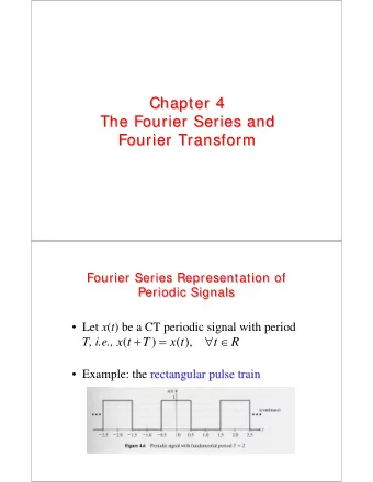
Numerical Fourier analysis of quasiperiodic functions G. Gmez, 1 - PowerPoint PPT Presentation

Fourier analysis Numerical Fourier analysis of quasi–periodic functions G. Gómez, 1 J.M. Mondelo 2 C. Simó 1 1 Departament de Matemàtica Aplicada i Anàlisi, Universitat de Barcelona 2 Departament de Matemàtiques, Universitat Autònoma de Barcelona WSIMS08 IMUB dec 1–5, 2008

Fourier analysis Outline Introduction The method Error estimation Accuracy test Study of the stability region around L 5

Fourier analysis Introduction Outline Introduction The method Error estimation Accuracy test Study of the stability region around L 5

Fourier analysis Introduction Setting We are given an analytic, quasi–periodic function � a k e i 2 π � k , ω � t , f ( t ) = k ∈ Z m satisfying the Cauchy estimates � � | a k | ≤ Ce − δ | k | ∃ C > 0 , δ > 0 , | k | = | ( k 1 , . . . , k m ) | = | k 1 | + · · · + | k m | and with a vector of basic frequencies ω = ( ω 1 , . . . , ω m ) satisfying a Diophantine condition � � |� k , ω �| > D ∃ D , τ > 0 | k | τ , . We want to numerically compute the frequencies {� k , ω �} maxor | k | = 0 and amplitudes a k from the values of f .

Fourier analysis Introduction Fourier Transform The Fourier Transform will be denoted as � ∞ � � F ( ω ) = ˆ f ( t ) e − i 2 πω t dt f ( t ) − → F f ( t ) f ( ω ) = −∞ If f ( t ) is quasi–periodic, its Fourier transform is a discrete set of impulses based at the frequencies: � � a k e i 2 π � k , ω � t F ˆ f ( t ) = − → f ( ω ) = a k δ � k , ω � ( ω ) k ∈ Z m k ∈ Z m 2 1.2 1.5 1 1 0.8 0.5 0.6 0 0.4 -0.5 0.2 -1 0 -1.5 -0.2 -20 -10 0 10 20 30 40 50 60 -0.6 -0.4 -0.2 0 0.2 0.4 0.6 Example: f ( t ) = cos ( 2 π 0 . 1 t ) + 0 . 5 cos ( 2 π 0 . 2 t ) + 0 . 4 cos ( 2 π 0 . 35 t )

Fourier analysis Introduction Time truncation − → WFT Graphical development (E.O. Brigham, 1988) Time truncation gives rise to the phenomenon known as leakage . Example: T = 40, f ( t ) = cos ( 2 π 0 . 1 t ) + 0 . 5 cos ( 2 π 0 . 2 t ) + 0 . 4 cos ( 2 π 0 . 35 t ) . 2 2 2 1.5 1.5 1.5 1 1 1 0.5 0.5 0.5 × → 0 0 0 -0.5 -0.5 -0.5 -1 -1 -1 -1.5 -1.5 -1.5 -20 -10 0 10 20 30 40 50 60 -20 -10 0 10 20 30 40 50 60 -20 -10 0 10 20 30 40 50 60 ↓ F ↓ F ↓ F 1.2 40 40 1 35 35 30 30 0.8 25 25 0.6 20 20 ∗ → 0.4 15 15 10 10 0.2 5 5 0 0 0 -0.2 -0.6 -0.4 -0.2 0 0.2 0.4 0.6 -0.6 -0.4 -0.2 0 0.2 0.4 0.6 -0.6 -0.4 -0.2 0 0.2 0.4 0.6 The maxima of the WFT (bottom right) are displaced from the true frequencies.

Fourier analysis Introduction Time truncation − → WFT Explicit formulae ◮ Windowed Fourier Transform: 1 � � φ f , T ( ω ) := T F χ [ 0 , T ] f ( t ) ( ω ) � T 1 χ [ 0 , T ] ( t ) f ( t ) e − i 2 πω t dt . = T 0 ◮ Leakage of a complex exponential term. � � e i 2 π ( ν − ω ) T − 1 � � � � | φ e i 2 πν t , T ( ω ) | = � � i 2 π ( ν − ω ) T � � � sin π ( ν − ω ) T � � � = � � π ( ν − ω ) T | sinc (( ν − ω ) T ) | =

Fourier analysis Introduction Reducing leackage There are two strategies: ◮ Increase the window length. � � � sin π ( ν − ω ) T � � � | φ e i 2 πν t , T ( ω ) | = | sinc (( ν − ω ) T ) | = � � π ( ν − ω ) T T=40 T=80 40 1 35 0.8 30 25 0.6 20 0.4 15 10 0.2 5 0 0 -0.6 -0.4 -0.2 0 0.2 0.4 0.6 -0.6 -0.4 -0.2 0 0.2 0.4 0.6

Fourier analysis Introduction Reducing leackage There are two strategies: ◮ Use a smoother window. We use Hanning’s: � � n h 1 − cos 2 π t H n h T ( t ) = q n h . T � � being q n h = n h ! / ( 2 n h − 1 )!! . The corresponding WFT is denoted by � T � � ( ω ) = 1 T ( t ) f ( t ) e − i 2 πω t dt , φ n h H n h f H n h f , T ( ω ) := F T 0

Fourier analysis Introduction Reducing leackage There are two strategies: ◮ Use a smoother window. � � e i 2 π ( ν − ω ) T − 1 1 φ e i 2 πν t , T ( ω ) = = O , i 2 π ( ν − ω ) T ( ν − ω ) T vs ( − 1 ) n h ( n h !) 2 � � � � e i 2 π ( ν − ω ) T − 1 1 φ n h e i 2 πν t , T ( ω ) = i 2 π � n h � � = O � � 1 + 2 n h ( ν − ω ) T + j ( ν − ω ) T j = − n h 1 n h =0 n h =0 1 n h =1 n h =1 0.8 0.1 n h =2 n h =2 | DFT | n h =3 | DFT | n h =3 0.01 0.6 0.001 0.4 0.0001 0.2 1e-05 0 1e-06 6 8 10 12 14 16 18 20 6 8 10 12 14 16 18 20 k k

Fourier analysis Introduction Discretization − → DFT Graphical development (E.O. Brigham, 1988) T = 40 , N = 32 , f ( t ) = cos ( 2 π 0 . 1 t ) + 0 . 5 cos ( 2 π 0 . 2 t ) + 0 . 4 cos ( 2 π 0 . 35 t ) 2 40 1.5 35 30 1 F 25 0.5 → 20 0 15 -0.5 10 5 -1 0 -1.5 0 10 20 30 40 -2 -1.6 -1.2 -0.8 -0.4 0 0.4 0.8 1.2 1.6 2 × ∗ impulse spacing = sampling rate = T/N = 1.25 impulse spacing = DFT period = N/T = 0.8 2 1 1.5 F 0.8 1 → 0.6 0.5 .... .... 0 0.4 -0.5 0.2 -1 0 -1.5 0 10 20 30 40 -2 -1.6 -1.2 -0.8 -0.4 0 0.4 0.8 1.2 1.6 2 ↓ ↓ 2 30 1.5 25 1 F 20 0.5 → 0 15 -0.5 10 -1 5 -1.5 0 0 10 20 30 40 -2 -1.6 -1.2 -0.8 -0.4 0 0.4 0.8 1.2 1.6 2

Fourier analysis Introduction Sampling − → DFT Explicit formulae ◮ DFT of { f ( j T N ) } N − 1 j = 0 defined as { F f , T , N ( k ) } N − 1 k = 0 , being �� �� k � � � � � 1 j T j T F f , T , N ( k ) := N F χ [ 0 , T ] f δ j T N N T N j ∈ Z N − 1 � � � 1 j T e − i 2 π kj / N . = f N N j = 0 ◮ With Hanning’s window: N − 1 � � � � � f , T , N ( k ) = 1 j T j T e − i 2 π kj / N . F n h H n h f T N N N j = 0

Fourier analysis Introduction Sampling − → DFT Explicit formulae ◮ Relation with the WFT: � � � k � � k + lN � k − lN � F f , T , N ( k ) = φ f , T , N + φ f , T , N ) + φ f , T , N ) T T T l ∈ Z \{ 0 } � �� � error term ◮ The fundamental domain of the DFT for real signals is [ 0 , T / ( 2 N )] . T / ( 2 N ) is Nyquist’s critical frequency. 1.2 1.2 1 1 0.8 0.8 0.6 0.6 0.4 0.4 0.2 0.2 0 0 -0.2 -0.2 -2 -1.6 -1.2 -0.8 -0.4 0 0.4 0.8 1.2 1.6 2 -2 -1.6 -1.2 -0.8 -0.4 0 0.4 0.8 1.2 1.6 2

Fourier analysis Introduction Sampling − → DFT Explicit formulae ◮ Relation with the WFT: � � � k � � k + lN � k − lN � F f , T , N ( k ) = φ f , T , N + φ f , T , N ) + φ f , T , N ) T T T l ∈ Z \{ 0 } � �� � error term ◮ The fundamental domain of the DFT for real signals is [ 0 , T / ( 2 N )] . T / ( 2 N ) is Nyquist’s critical frequency. ◮ The error term above can produce aliasing : if a frequency of the signal is outside the fundamental domain of the DFT, we will detect an alias of it. ◮ Aliasing is avoided increasing N .

Fourier analysis The method Outline Introduction The method Error estimation Accuracy test Study of the stability region around L 5

Fourier analysis The method Algorithm Parameters: T (time length), N (number of samples), n h (Hanning index) b min minimum threshold, several tolerances. 1. Set an starting threshold for collecting peaks of the modulus of the DFT of f ( t ) . 2. Find initial approximations of the frequencies , starting from the peaks of the DFT greater than the thresold. 3. Find the amplitudes of the frequencies found in the previous step, by solving DFT ( Q f ) = DFT ( f ) . 4. Simultaneously refine ALL the frequencies and amplitudes of the current quasi–periodic approximation of f , by solving DFT ( Q f ) = DFT ( f ) . 5. Perform a DFT of the input signal minus the current quasi–periodic approximation obtained in step 4, decrease the thresold and go back to step 2 .

Fourier analysis The method Algorithm Parameters: T (time length), N (number of samples), n h (Hanning index) b min minimum threshold, several tolerances. 1. Set an starting threshold for collecting peaks of the modulus of the DFT of f ( t ) . 2. Find initial approximations of the frequencies , starting from the peaks of the DFT greater than the thresold. 3. Find the amplitudes of the frequencies found in the previous step, by solving DFT ( Q f ) = DFT ( f ) . 4. Simultaneously refine ALL the frequencies and amplitudes of the current quasi–periodic approximation of f , by solving DFT ( Q f ) = DFT ( f ) . 5. Perform a DFT of the input signal minus the current quasi–periodic approximation obtained in step 4, decrease the thresold and go back to step 2 .

Fourier analysis The method Algorithm Parameters: T (time length), N (number of samples), n h (Hanning index) b min minimum threshold, several tolerances. 1. Set an starting threshold for collecting peaks of the modulus of the DFT of f ( t ) . 2. Find initial approximations of the frequencies , starting from the peaks of the DFT greater than the thresold. 3. Find the amplitudes of the frequencies found in the previous step, by solving DFT ( Q f ) = DFT ( f ) . 4. Simultaneously refine ALL the frequencies and amplitudes of the current quasi–periodic approximation of f , by solving DFT ( Q f ) = DFT ( f ) . 5. Perform a DFT of the input signal minus the current quasi–periodic approximation obtained in step 4, decrease the thresold and go back to step 2 .