GLM and GAMs Workshop By Aaron Greenville Stats model - PowerPoint PPT Presentation

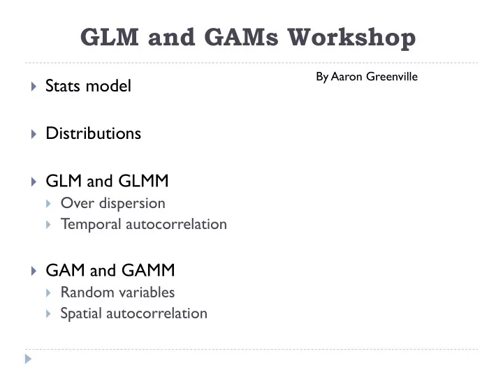
GLM and GAMs Workshop By Aaron Greenville  Stats model  Distributions  GLM and GLMM  Over dispersion  T emporal autocorrelation  GAM and GAMM  Random variables  Spatial autocorrelation

Stats model DETERMINISTIC STOCHASTIC mass i = α + β x Sex i + ε i Constants We are used to ε i following a normal distribution Remember linear equation...

Beyond the normal distribution Continuous distributions Discrete distributions

Generalized linear models (GLM) We choose the distribution the error (stochastic part) follows. Hence • Generalized. Very powerful as they are flexible • Binomial regression - the probability of a success is related to • explanatory variables: the corresponding concept in ordinary regression is to relate the mean value of the unobserved response to explanatory variables. • Logistic regression - is used for prediction of the probability of occurrence of an event by fitting data to a logistic curve. Special case of binomial regression Poisson or negative binomial models • Zero-inflated models •

GLM cont.  Quasi-distributions  Can have random variables, nested designs etc  Can use traditional hypothesis testing  Or model selection techniques ( AICc’s etc)  Can use Bayesian methods

GLM cont.  Link function  Specify the relationship of the response variable (y) and deterministic part (predictor variables)  So GLM has 3 parts  Data follows some dist e.g mass follows Poisson, mean = variance.  Link between mean of y (mass) and predictor variable(s). E.g. Log for poisson  Deterministic part: log(mean mass i )= α + β x Sex i  Deviance = (null deviance – residual deviance)/null deviance

Poisson GLM example: Frog roadkill Exercise 5: 1. No. of frogs killed follows Poisson dist 2. log link function needed 3. log(mean frogsKilled)= α + β x Dist.Park+ ε i

GLM cont.: Frog road kill

Poisson GLM example: Frog roadkill Not linear because of glm(formula = TOT.N ~ D.PARK, family = poisson, data = RK) the log link function Deviance Residuals: Min 1Q Median 3Q Max -8.1100 -1.6950 -0.4708 1.4206 7.3337 α Coefficients: Estimate Std. Error z value Pr(>|z|) (Intercept) 4.316e+00 4.322e-02 99.87 <2e-16 *** D.PARK -1.059e-04 4.387e-06 -24.13 <2e-16 *** --- Signif . codes: 0 ‘***’ 0.001 ‘**’ 0.01 ‘*’ 0.05 ‘.’ 0.1 ‘ ’ 1 β ( Dispersion parameter for poisson family taken to be 1 ) Null deviance: 1071.4 on 51 degrees of freedom Residual deviance: 390.9 on 50 degrees of freedom AIC: 634.29 Looks like over-dispersion ~64% deviance explained here

GLM cont.: model checking

Quasi-poisson GLM glm(formula = TOT.N ~ D.PARK, family = quasipoisson, data = RK) Deviance Residuals: Min 1Q Median 3Q Max -8.1100 -1.6950 -0.4708 1.4206 7.3337 Coefficients: Estimate Std. Error t value Pr(>|t|) (Intercept) 4.316e+00 1.194e-01 36.156 < 2e-16 *** D.PARK -1.058e-04 1.212e-05 -8.735 1.24e-11 *** --- Signif . codes: 0 ‘***’ 0.001 ‘**’ 0.01 ‘*’ 0.05 ‘.’ 0.1 ‘ ’ 1 ( Dispersion parameter for quasipoisson family taken to be 7.630148 ) Null deviance: 1071.4 on 51 degrees of freedom Residual deviance: 390.9 on 50 degrees of freedom AIC: NA

GLM cont.: model checking

Neg bin GLM: Frog road kill glm.nb(formula = TOT.N ~ D.PARK, data = RK, link = "log", init.theta = 3.681040094) Deviance Residuals: Min 1Q Median 3Q Max -2.4160 -0.8289 -0.2116 0.4800 2.1346 Coefficients: Estimate Std. Error z value Pr(>|z|) (Intercept) 4.411e+00 1.548e-01 28.50 <2e-16 *** D.PARK -1.161e-04 1.137e-05 -10.21 <2e-16 *** --- Signif . codes: 0 ‘***’ 0.001 ‘**’ 0.01 ‘*’ 0.05 ‘.’ 0.1 ‘ ’ 1 (Dispersion parameter for Negative Binomial(3.681) family taken to be 1) Null deviance: 155.445 on 51 degrees of freedom Residual deviance: 54.742 on 50 degrees of freedom AIC: 393.09 Better Number of Fisher Scoring iterations: 1 Theta: 3.681 Std. Err.: 0.891 ~65% deviance explained

GLM cont.: model checking

GLMM with temporal confounding Exercise 6:  Hawaii birds abundance over time  Normal dist with identity link function  Mean birds = α + β x Year+ β 2 Rainfall+ ε i

GLMM: Bird e.g cont.

GLMM: Birds e.g. cont. Generalized least squares fit by REML Model: Birds ~ Rainfall + Year Data: Hawaii AIC BIC logLik 228.4798 235.4305 -110.2399 Coefficients: Value Std.Error t-value p-value (Intercept) -477.66 56.41907 -8.466346 0.0000 Rainfall 0.0009 0.04989 0.017245 0.9863 Year 0.2450 0.02847 8.604858 0.0000

GLMM cont. Note pattern

Looking for temporal autocorrelation  Oh Dear! Oh dear!

GLMM cont.  Need to take into account temporal autocorrelation/confounding  Lots of variance structures you can use.  corAR1: Says data 1 yr apart is more correlated than 2 yrs apart, 3 yrs apart etc. So after x number of years there will be no correlation.  corARMA: autoregressive moving average process, with arbitrary orders for the autoregressive and moving average components.  corCAR1: continuous autoregressive process (AR(1) process for a continuous time covariate).  corCompSymm: compound symmetry structure corresponding to a constant correlation.

GLMM cont. Generalized least squares fit by REML Model: Birds ~ Rainfall + Year AIC lower Data: Hawaii AIC BIC logLik 199.1394 207.8277 -94.5697 Correlation Structure: ARMA(1,0) Formula: ~Year Parameter estimate(s): Residuals separated by 1 yr are Phi1 correlated at 0.77, 2 yrs 0.77 2 etc 0.7734303 Coefficients: Value Std.Error t-value p-value p-value not as (Intercept) -436.4326 138.74948 -3.145472 0.0030 sign. Rainfall -0.0098 0.03268 -0.300964 0.7649 Year 0.2241 0.07009 3.197828 0.0026

Generalized Additive Models  More general again! Can do similar things to GLM.  Fit a model using smoothing techniques, so they follow the data very closely.  Non-Linear  Problem: you can fit a great model to the data, but is it meaningful.

GAM cont.  GAM has 3 parts  Data follows some dist e.g mass follows Poisson, mean = variance.  Link between mean of y (mass) and predictor variable(s). E.g. Log for poisson  Deterministic part: log(mean roadkill)= α + f (Dist.Park) Smoother function

Example GAM smoother

GAMM: Spatial autocorrelation shapes Ratio Spherical Linear Exponential Gaussian

Steps to choosing appropriate analysis  What type of data is it? i.e. What distribution is most appropriate?  Is the relationship linear or non-linear?  Does the model have random variables, spatial or temporal confounding?

Further Reading