Number of solutions to a linear system We just proved: If u 1 is a - PowerPoint PPT Presentation

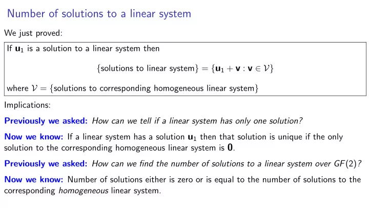
Number of solutions to a linear system We just proved: If u 1 is a solution to a linear system then { solutions to linear system } = { u 1 + v : v ∈ V} where V = { solutions to corresponding homogeneous linear system } Implications: Previously we asked: How can we tell if a linear system has only one solution? Now we know: If a linear system has a solution u 1 then that solution is unique if the only solution to the corresponding homogeneous linear system is 0 . Previously we asked: How can we find the number of solutions to a linear system over GF (2) ? Now we know: Number of solutions either is zero or is equal to the number of solutions to the corresponding homogeneous linear system.

Number of solutions: checksum function A checksum function maps long files to short sequences. Idea: I Web page shows the checksum of each file to be downloaded. I Download the file and run the checksum function on it. I If result does not match checksum on web page, you know the file has been corrupted. I If random corruption occurs, how likely are you to detect it? Impractical but instructive checksum function: I input: an n -vector x over GF (2) I output: [ a 1 · x , a 2 · x , . . . , a 64 · x ] where a , a , . . . , a are sixty-four n -vectors.

Number of solutions: checksum function Our checksum function: I input: an n -vector x over GF (2) I output: [ a 1 · x , a 2 · x , . . . , a 64 · x ] where a 1 , a 2 , . . . , a 64 are sixty-four n -vectors. Suppose p is the original file, and it is randomly corrupted during download. What is the probability that the corruption is undetected? The checksum of the original file is [ β 1 , . . . , β 64 ] = [ a 1 · p , . . . , a 64 · p ]. Suppose corrupted version is p + e . Then checksum of corrupted file matches checksum of original if and only if a 1 · ( p + e ) = β 1 a 1 · p − a 1 · ( p + e ) = 0 a 1 · e = 0 i ff i ff . . . . . . . . . a 64 · ( p + e ) = a 64 · p − a 64 · ( p + e ) = 0 a 64 · e = 0 β 64 i ff e is a solution to the homogeneous linear system a 1 · x = 0 , . . . a 64 · x = 0.

Number of solutions: checksum function Suppose corrupted version is p + e . Then checksum of corrupted file matches checksum of original if and only if e is a solution to homogeneous linear system a 1 · x = 0 . . . a 64 · x = 0 If e is chosen according to the uniform distribution, Probability ( p + e has same checksum as p ) = Probability ( e is a solution to homogeneous linear system) number of solutions to homogeneous linear system = number of n -vectors number of solutions to homogeneous linear system = 2 n Question: How to find out number of solutions to a homogeneous linear system over GF (2)?

Geometry of sets of vectors: convex hull Earlier, we saw: The u -to- v line segment is { α u + β v : α ∈ R , β ∈ R , α ≥ 0 , β ≥ 0 , α + β = 1 } Definition: For vectors v 1 , . . . , v n over R , a linear combination α 1 v 1 + · · · + α n v n is a convex combination if the coe ffi cients are all nonnegative and they sum to 1. I Convex hull of a single vector is a point. I Convex hull of two vectors is a line segment. I Convex hull of three vectors is a triangle Convex hull of more vectors? Could be higher-dimensional... but not necessarily. For example, a convex polygon is the convex hull of its vertices

Activity: Vec You wrote the procedures in vec.py : add(u,v), scalar mul(alpha, v), neg(v), dot(u,v) Try writing these I without using setitem or v[k] = ... I without doing any mutation I without assigning more than once to any variable (aside from comprehensions)

Two kinds of functions Focus on two kinds of functions: I dot-product functions I linear-combination functions Dot-product function: I A function is specified by some C -vectors a 1 , . . . , a m I Input is a C -vector x I Output is [ a 1 · x , . . . , a m · x ] Linear-combination function: I A function is specified by some R -vectors v 1 , . . . , v n I Input is a list of n scalars [ α 1 , . . . , α n ] I Output is α 1 v 1 + · · · + α n v n

Example applications of dot-product function I Cost/benefit I C = { malt , hops , yeast , water } cost vector a 1 = { hops : $2 . 50 / ounce , malt : $1 . 50 / pound , water : $0 . 06 / gallon , yeast : $ . 45 / g } calorie vector a 2 = { hops : 0 , malt : 960 , water : 0 , yeast : 3 . 25 } input x specifies quantity of each ingredient for some recipe, e.g. x = { hops:6 oz, malt:14 pounds, water:7 gallons, yeast:11 grams } I Consumption of resources C = { radio , sensor , memory , CPU } a 1 is a vector specifying how long each hardware component is working during test period 1 . . . a m is a vector specifying how long each hardware component is working during test period m x specifies how much energy each component consumes per second, e.g. x = { memory : 0 . 06W , radio : 0 . 06W , sensor : 0 . 004W , CPU : 0 . 0025W } function f ( x ) = [ a 1 · x , . . . , a m · x ] maps energy consumption per component to total energy consumption per test period.

More example applications of dot-product functions I match filter (image or audio search) C is set of audio sample times or pixel locations For each possible location of match, have a vector a i x is an digital audio recording or a digital image. f ( x ) = [ a 1 , . . . , a m ] maps x to measurements of closeness of match I Authentication C = { 0 , . . . , n − 1 } Each a i is a challenge observed by Eve x is password f ( x ) = [ a 1 · x , . . . , a m · x ] maps x to the list of responses Eve observed.

Applications of dot-product definition: Downsampling I Each pixel of the low-res image corresponds to a little grid of pixels of the high-res image. I The intensity value of a low-res pixel is the average of the intensity values of the corresponding high-res pixels.

Applications of dot-product functions: Downsampling I Each pixel of the low-res image corresponds to a little grid of pixels of the high-res image. I The intensity value of a low-res pixel is the average of the intensity values of the corresponding high-res pixels. I Averaging can be expressed as dot-product. I We want to compute a dot-product for each low-res pixel.

Applications of dot-product functions: blurring I To blur a face, replace each pixel in face with average of pixel intensities in its neighborhood. I Average can be expressed as dot-product. I Gaussian blur: a kind of weighted average

Applications of linear combinations Resource consumption profile For making one gnome: v 1 = { metal:0, concrete:1.3, plastic:0.2, water:0.8, electricity:0.4 } For making one hula hoop: v 2 = { metal:0, concrete:0, plastic:1.5, water:0.4, electricity:0.3 } For making one slinky: v 3 = { metal:0.25, concrete:0, plastic:0, water:0.2, electricity:0.7 } For making one silly putty: v 4 = { metal:0, concrete:0, plastic:0.3, water:0.7, electricity:0.5 } For making one salad shooter: v 5 = { metal:1.5, concrete:0, plastic:0.5, water:0.4, electricity:0.8 } input [number α 1 of gnomes, number α 2 of hula hoops, ..., number α 5 of salad shooters] function f ([ α 1 , α 2 , α 3 , α 4 , α 5 ] = α 1 v 1 + α 2 v 2 + α 3 v 3 + α 4 v 4 + α 5 v 5 outputs the total resource consumption profile.

Applications of linear combinations Lights Out (over GF (2) • • • • • • vectors v 1 , . . . , v n are button vectors, e.g. • • • • • • x = [ α 1 , . . . , α n ] specifies whether a button is pressed or not f ([ α 1 , . . . , α n ]) = α 1 v 1 + · · · + α n v n specifies what initial state this solves