Notes on Transformations and Generalized Linear Models W N Venables - PDF document

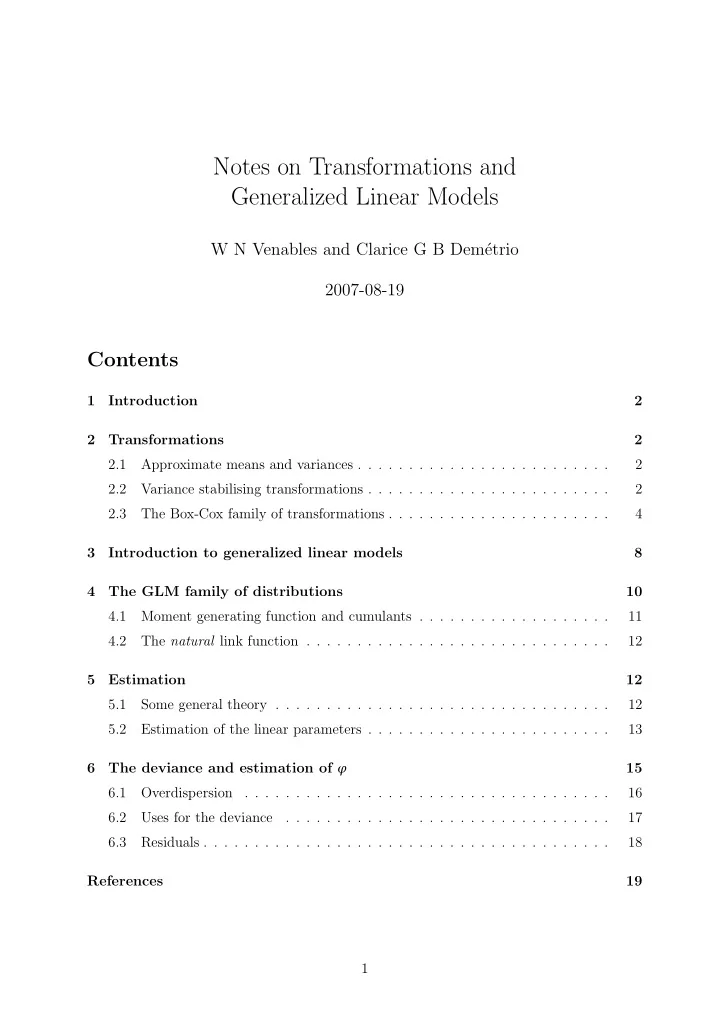
Notes on Transformations and Generalized Linear Models W N Venables and Clarice G B Dem´ etrio 2007-08-19 Contents 1 Introduction 2 2 Transformations 2 2.1 Approximate means and variances . . . . . . . . . . . . . . . . . . . . . . . . . 2 2.2 Variance stabilising transformations . . . . . . . . . . . . . . . . . . . . . . . . 2 2.3 The Box-Cox family of transformations . . . . . . . . . . . . . . . . . . . . . . 4 3 Introduction to generalized linear models 8 4 The GLM family of distributions 10 4.1 Moment generating function and cumulants . . . . . . . . . . . . . . . . . . . 11 4.2 The natural link function . . . . . . . . . . . . . . . . . . . . . . . . . . . . . . 12 5 Estimation 12 5.1 Some general theory . . . . . . . . . . . . . . . . . . . . . . . . . . . . . . . . . 12 5.2 Estimation of the linear parameters . . . . . . . . . . . . . . . . . . . . . . . . 13 6 The deviance and estimation of ϕ 15 6.1 Overdispersion . . . . . . . . . . . . . . . . . . . . . . . . . . . . . . . . . . . . 16 6.2 Uses for the deviance . . . . . . . . . . . . . . . . . . . . . . . . . . . . . . . . 17 6.3 Residuals . . . . . . . . . . . . . . . . . . . . . . . . . . . . . . . . . . . . . . . . 18 References 19 1

1 Introduction These notes are intended to provide an introduction to generalized linear modelling, em- phasising the way relationship between the modern theory and the older theory of trans- formations, out of which the idea developed. We consider transformations in statistics, however, to be of much more than historical interest. The brief treatment we give here is intended to be as much for their use in contemporary data analysis as for showing the origins of the idea of a generalized linear model. 2 Transformations 2.1 Approximate means and variances Let Y be a random variable with first two moments � ( Y − µ ) 2 � = σ 2 . E [ Y ] = µ and var [ Y ] = E Now let U = g ( Y ) be another random variable defined as a function of Y and we need an ap- proximate expression for its first two moments as well. If we can assume that g ( . ) is smooth and only slowly varying, at least in the region where its argument, Y , is stochastically lo- cated, the simplest approach to this problem is to assume that a linear approximation to g ( . ) near the mean of Y is adequate. Expanding g ( . ) in a Taylor series gives U = g ( Y ) = g ( µ ) + g ′ ( µ )( Y − µ ) + “smaller order terms” Neglecting the smaller order terms gives the approximate expressions � � g ( µ ) + g ′ ( µ ) E E [ U ] (1) ≈ ( Y − µ ) = g ( µ ) �� � 2 � � ( Y − µ ) 2 � ≈ g ′ ( µ ) 2 E = g ′ ( µ ) 2 σ 2 var [ U ] E (2) ≈ U − g ( µ ) Approximate formulae 1 and 2, and extensions to them, are often referred to in statistics as “the delta method”. They are useful in their own right, but they also give some elementary guidance about the possible choices of transformation to achieve various aims. 2.2 Variance stabilising transformations If the variance of Y is not constant but changes with the mean, that is var [ Y ] = σ 2 ( µ ) , this can often cause difficulties with both interpretation and analysis. In these cases one possible way around the difficulties might be to transform the response, Y , to a new scale in which the variance is at least approximately constant. Suppose, then, that we transform the response to U = g ( Y ) . The delta method suggests that if we want the variance of U to be approximately constant, then we should choose g ( . ) such that var [ g ( Y )] ≈ g ′ ( µ ) 2 σ 2 ( µ ) = k 2 2

where k is a constant. In other words, we should choose g ( . ) to be any solution of g ′ ( t ) = dg k dt = σ ( t ) up to changes in location and scale. A convenient solution, then, is � y dt g ( y ) = σ ( t ) Example 2.1 If Y has a Poisson distribution, Y ∼ Po( µ ) , then E [ Y ] = var [ Y ] = µ = σ 2 ( µ ) To transform the distribution to approximately constant variance, then, the suggested transform is � y dt � y dt = 2 � y g ( y ) = σ ( t ) = � t Taking the square root was a standard technique in the analysis of count data and towards the middle of the last century much work was done to refine it. Example 2.2 Suppose S is a Binomial random variable, S ∼ B( n , ̟ ) , and put Y = S / n , the ’proportion of successes’. Then var [ Y ] = σ 2 ( µ ) = µ (1 − µ ) E [ Y ] = ̟ = µ , n Hence, up to location and scale, the suggested transformation that will approximately stabilise the variance is � y dt � y � n dt � n sin − 1 � y g ( y ) = σ ( t ) = � = t (1 − t ) Transforming with an ‘arc-sine square-root’ was a standard technique in the analysis of proportion data and, as in the Poisson case, much work was done to refine it prior to the general adoption of generalised linear modelling alternatives. Example 2.3 A distribution for which the ratio cv = σ / µ = k is constant with respect to the mean is said to have “constant coefficient of variation”. Since σ 2 ( µ ) = k 2 µ 2 , the suggested transformation to stabilise the variance is � y dt � y dt σ ( t ) = 1 t = 1 g ( y ) = k log( y ) k Hence for such distributions the log transformation is suggested to make the variance at least approximately constant with respect to the mean. As an exercise, show that both the gamma and lognormal distributions have constant coefficient of variation, and examine to what extent the log transformation stabilises the variance with respect to the mean. The gamma distribution has probability density function f Y ( y ; α , φ ) = e − y / α y φ − 1 α φ Γ ( φ ) , 0 < y < ∞ The lognormal distribution is defined by transformation. We say Y has a lognormal dis- tribution if log Y ∼ N ( µ , σ 2 ) . 3

2.3 The Box-Cox family of transformations Transforming a response to stabilise the variance will, of course, also affect the relationship between the mean and the candidate predictors. In a pioneering paper [Box & Cox(1964)] Box and Cox suggested a method for choosing a transformation that allowed the effect on both the mean and the variance to be taken into account. They considered a family of transformations defined by  y λ − 1   λ �= 0 dg ( y ; λ ) = y λ − 1 λ with g ( y ; λ ) =  dy  log y λ = 0 Note that this includes both the square-root and log transformations, along with other power transformations which are often used in practice, (including the trivial identity transformation). Now suppose we have a sample of responses and that after transformation it conforms to a linear model specification as follows (with an obvious notation): � � X β , σ 2 I n g ( y ; λ ) ∼ N The likelihood function for the sample is the distribution of y , namely 2 log( σ 2 ) − � g ( y ; λ ) − X β � 2 � n log L ( β , σ 2 , λ ; y ) = − n 2 log(2 π ) − n y λ − 1 + log i 2 σ 2 i = 1 where the final term on the right is the Jacobian factor for the inverse transformation. (This is only an approximate result in general as for most transformations in the family the range is not −∞ < y < ∞ , but we ignore this here.) Maximising this with respect to β and σ 2 gives the profile likelihood for λ , which by standard results is easily shown to be � � � n log L = − n 2 log(2 π / n ) − n − n log L ⋆ ( λ ; y ) = max g ( y ; λ ) T ( I − P X ) g ( y ; λ ) y λ − 1 2 log 2 + log i β , σ 2 | λ i = 1 where P X = X ( X T X ) − X T is the orthogonal projector matrix on to the range of X , and the quantity in braces, { ... } , is the residual sum of squares after regressing the transformed response on X . As pointed out by Box and Cox, the Jacobian factor can be combined with RSS term in a neat way. Note that � n = n y λ − 1 y 2( λ − 1) log 2 log ˙ i i = 1 �� n � 1/ n is the geometric mean of the observations. Now define a slightly where ˙ y = i = 1 y i modified response as � y λ − 1 z ( λ ) = g ( y ; λ ) ˙ Then the profile likelihood for λ may be written � � log L ⋆ ( λ ; y ) = const. − n z ( λ ) T ( I − P X ) z ( λ ) 2 log 4