News Review: Collision Proxy Tradeoffs Review: Spatial Data - PowerPoint PPT Presentation

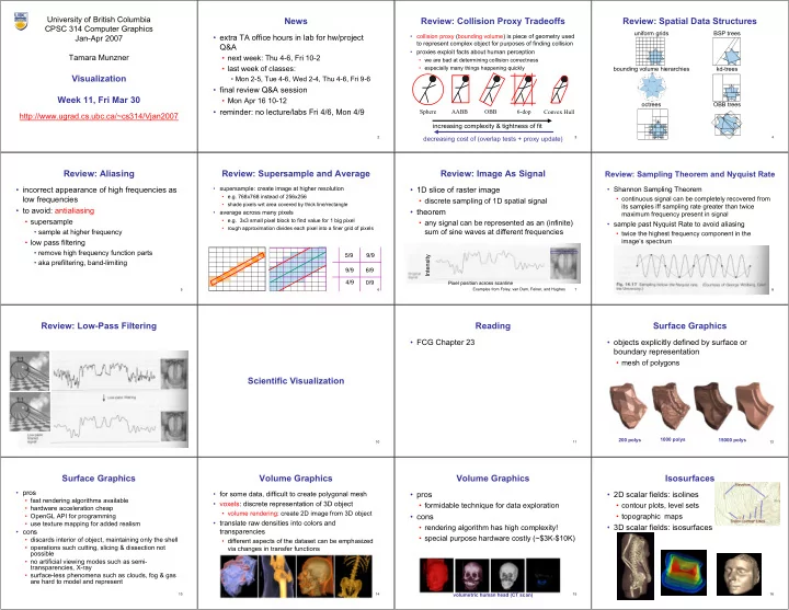
University of British Columbia News Review: Collision Proxy Tradeoffs Review: Spatial Data Structures CPSC 314 Computer Graphics uniform grids BSP trees • extra TA office hours in lab for hw/project • collision proxy (bounding volume) is piece of geometry used Jan-Apr 2007 to represent complex object for purposes of finding collision Q&A • proxies exploit facts about human perception Tamara Munzner • next week: Thu 4-6, Fri 10-2 • we are bad at determining collision correctness • last week of classes: • especially many things happening quickly bounding volume hierarchies kd-trees Visualization • Mon 2-5, Tue 4-6, Wed 2-4, Thu 4-6, Fri 9-6 • final review Q&A session Week 11, Fri Mar 30 • Mon Apr 16 10-12 octrees OBB trees • reminder: no lecture/labs Fri 4/6, Mon 4/9 Sphere AABB OBB 6-dop Convex Hull http://www.ugrad.cs.ubc.ca/~cs314/Vjan2007 increasing complexity & tightness of fit decreasing cost of (overlap tests + proxy update) 2 3 4 Review: Aliasing Review: Supersample and Average Review: Image As Signal Review: Sampling Theorem and Nyquist Rate • incorrect appearance of high frequencies as • supersample: create image at higher resolution • 1D slice of raster image • Shannon Sampling Theorem • e.g. 768x768 instead of 256x256 low frequencies • continuous signal can be completely recovered from • discrete sampling of 1D spatial signal • shade pixels wrt area covered by thick line/rectangle its samples iff sampling rate greater than twice • to avoid: antialiasing • theorem • average across many pixels maximum frequency present in signal • supersample • e.g. 3x3 small pixel block to find value for 1 big pixel • any signal can be represented as an (infinite) • sample past Nyquist Rate to avoid aliasing • rough approximation divides each pixel into a finer grid of pixels sum of sine waves at different frequencies • sample at higher frequency • twice the highest frequency component in the image’s spectrum • low pass filtering • remove high frequency function parts 5/9 9/9 Intensity • aka prefiltering, band-limiting 9/9 6/9 4/9 0/9 Pixel position across scanline Examples from Foley, van Dam, Feiner, and Hughes 5 6 7 8 Review: Low-Pass Filtering Reading Surface Graphics • FCG Chapter 23 • objects explicitly defined by surface or boundary representation • mesh of polygons Scientific Visualization 200 polys 1000 polys 15000 polys 9 10 11 12 Surface Graphics Volume Graphics Volume Graphics Isosurfaces • pros • for some data, difficult to create polygonal mesh • pros • 2D scalar fields: isolines • fast rendering algorithms available • voxels: discrete representation of 3D object • formidable technique for data exploration • contour plots, level sets • hardware acceleration cheap • volume rendering: create 2D image from 3D object • OpenGL API for programming • cons • topographic maps • translate raw densities into colors and • use texture mapping for added realism • rendering algorithm has high complexity! • 3D scalar fields: isosurfaces transparencies • cons • special purpose hardware costly (~$3K-$10K) • discards interior of object, maintaining only the shell • different aspects of the dataset can be emphasized • operations such cutting, slicing & dissection not via changes in transfer functions possible • no artificial viewing modes such as semi- transparencies, X-ray • surface-less phenomena such as clouds, fog & gas are hard to model and represent volumetric human head (CT scan) 13 14 15 16

Volume Graphics: Examples Isosurface Extraction MC 1: Create a Cube MC 2: Classify Each Voxel • array of discrete point • consider a cube defined by eight data values • classify each voxel according to whether lies 0 1 1 3 2 samples at grid points • outside the surface (value > iso-surface • 3D array: voxels value) 1 3 6 6 3 • find contours (i,j+1,k+1) (i+1,j+1,k+1) • inside the surface (value <= iso-surface value) 10 10 3 7 9 7 3 • closed, continuous industrial CT - structural failure, Iso=9 anatomical atlas from visible (i,j,k+1) (i+1,j,k+1) security applications 5 5 human (CT & MRI) datasets • determined by iso-value 2 7 8 6 2 • several methods 10 8 Iso=7 • marching cubes is most (i,j+1,k) (i+1,j+1,k) 1 2 3 4 3 8 8 =inside common Iso-value = 5 =outside (i,j,k) (i+1,j,k) shockwave visualization: simulation flow around airplane wing with Navier-Stokes PDEs 17 18 19 20 MC 3: Build An Index MC 4: Lookup Edge List MC 4: Example MC 5: Interpolate Triangle Vertex • binary labeling of each voxel to create index • use index to access array storing list of edges • index = 00000001 • for each triangle edge • all 256 cases can be derived from 15 base • triangle 1 = a, b, c • find vertex location along edge using linear cases interpolation of voxel values c a i+1 i x v8 v7 11110100 inside =1 b v4 outside=0 v3 =10 =0 v5 v6 00110000 [] T v i T=8  −  v1 v2 Index: T=5 x i = +    ] []  [ v i 1 v i v1 v2 v3 v4 v5 v6 v7 v8 + −   21 22 23 24 MC 6: Compute Normals MC 7: Render! Rendering Pipeline Direct Volume Rendering • calculate the normal at each cube vertex • do not compute surface • use linear interpolation to compute the Classify polygon vertex normal G v v = − x i 1 , j , k i 1 , j , k + − G v v = − y i , j 1 , k i , j 1 , k + − G v v = − z i , j , k 1 i , j , k 1 + − 25 26 27 28 Classification Transfer Functions Transfer Functions Setting Transfer Functions • data set has application-specific values • map data value to color and opacity • can be difficult, unintuitive, and slow RGB α • temperature, velocity, proton density, etc. α • assign these to color/opacity values to make f α sense of data α ( f ) RGB( f ) f • achieved through transfer functions f α α shading, f compositing… f Gordon Kindlmann 29 30 Human Tooth CT 31 32 Gordon Kindlmann

Rendering Pipeline Light Effects Rendering Pipeline Interpolation 2D 1D • usually only consider reflected part • given: • given: Classify Light Classify reflected specular Light Shade Shade absorbed ambient • needed: diffuse • needed: transmitted Interpolate linear nearest Light=refl.+absorbed+trans. Light=ambient+diffuse+specular neighbor I k I k I k I = + + a a d d s s 33 34 35 36 Rendering Pipeline Volume Rendering Algorithms Ray Traversal Schemes Ray Traversal - First • ray casting • first: extracts iso-surfaces (again!) Intensity • image order, forward viewing Max Classify • splatting Intensity Average • object order, backward viewing Shade • texture mapping Accumulate Interpolate First First • object order • back-to-front compositing Composite Depth Depth 37 38 39 40 Ray Traversal - Average Ray Traversal - MIP Ray Traversal - Accumulate Splatting • average: looks like X-ray • max: Maximum Intensity Projection • accumulate: make transparent layers visible • each voxel represented as fuzzy ball • used for Magnetic Resonance Angiogram • 3D gaussian function • RGBa value depends on transfer function Intensity Intensity Intensity • fuzzy balls projected on screen, leaving Max footprint called splat Average • composite front to back, in object order Accumulate Depth Depth Depth 41 42 43 44 Texture Mapping InfoVis Example: TreeJuxtaposer • 2D: axis aligned 2D textures • side by side comparison of evolutionary trees • back to front compositing • stretch and squish navigation • commodity hardware support • guaranteed visibility • must calculate texture • progressive rendering coordinates, warp to image • demo - downloadable from http://olduvai.sf.net/tj plane • 3D: image aligned 3D texture • simple to generate texture coordinates 45 46