New computational methods for NLO and NNLO calculations in QCD - PowerPoint PPT Presentation

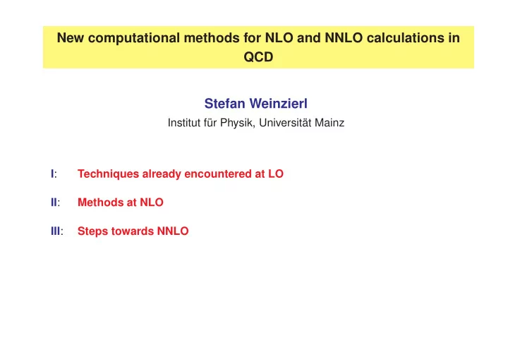
New computational methods for NLO and NNLO calculations in QCD Stefan Weinzierl Institut für Physik, Universität Mainz I : Techniques already encountered at LO II : Methods at NLO III : Steps towards NNLO

Part I: Prelude Physics is about numbers

Monte Carlo integration We are interested in multi-dimensional integrals: � d n u f ( u 1 ,..., u n ) = I [ 0 , 1 ] n Evaluate the integrand at N random points � u j = ( u j , 1 ,..., u j , n ) . N 1 ∑ = f ( � u j ) I N j = 1 Error scales as 1 σ ∼ √ N

Simulation of scattering events parton hadronisation and decay pdf’s hard scattering shower Underlying event: Interactions of the proton remnants. Multiple interactions: more than one pair of partons undergo hard scattering Pile-up events: more than one hadron-hadron scattering within a bunch crossing

Fixed-order calculations Done at the parton level with quarks and gluons. Usually only a few partons in the final state. Amplitudes calculated in perturbation theory. Method of choice to describe well-separated jets. pdf’s hard scattering

The master formula for the calculation of observables 1 1 � � = ∑ � O � dx 1 f a ( x 1 ) dx 2 f b ( x 2 ) n spin n spin 2 K ( ˆ s ) n colour n colour a a , b a b b � �� � � �� � � �� � pdf’s flux factor average over initial spins and colours � | A n + 2 | 2 × ∑ d φ n O ( p 1 ,..., p n ) � �� � � �� � n � �� � observable amplitude integral over phase space We will discuss: • Required properties of observables • Calculation of the amplitude • Integration over the phase space

Part I Infrared-safe observables

Soft and collinear particles A particle detector has a finite resolution. • Finite angular resolution: A pair of particles moving in (almost) the same direction can not be resolved below a certain angle. We call these particles a pair of collinear particles. Example: An electron and a photon not resolved by the electromagnetic calorimeter. • Detection only above a certain threshold: A particle with an energy below a certain threshold will not be detected. We call this particle a soft particle. Example: A low-energy photon.

Infrared-safe observables Observables which do not depend on long-distance behaviour, are called infrared-safe observables and can reliably be calculated in perturbation theory. In particular, it is required that they do not change value, if infinitessimal soft or collinear particles are added. For example: collinear : p i || p j O n ( p 1 ,..., p i ,..., p j ,..., p n ) = O n − 1 ( p 1 ,..., p ij ,..., p n ) lim soft : p j → 0 O n ( p 1 ,..., p j ,..., p n ) = O n − 1 ( p 1 ,..., p j − 1 , p j + 1 ,..., p n ) lim

Event shapes Event shapes are observables calculated from all particles in an event. Typical examples of infrared-safe event shapes in electron-positron annihilation are thrust, heavy jet mass, wide jet broadening, total jet broadening, C parameter, etc. Definition: Thrust i | � p i · ˆ n | ∑ = max T i | � p i | ∑ n ˆ For two particles back-to-back one has T = 1 For many particles, isotropically distributed we have T = 1 2

Spherocity versus sphericity Spherocity:   2 p ⊥ i | � i | ∑ � 4 � 2 = min S   π i | � p i | ∑ n ˆ Sphericity: p ⊥ i | 2 i | � ∑ � 4 � 2 min π i | � p i | 2 ∑ n ˆ Sphericity is not infrared-safe ! (Altarelli, Phys. Rept. 1981) ... however this does not stop experimentalists from measuring it ... (Aleph 1990)

Jet algorithms The most fine-grained look at hadronic events consistent with infrared safety is given by classifying the particles into jets. Ingredients for a sequential recombination algorithm: • a resolution variable y ij where a smaller y ij means that particles i and j are “closer”; 2 ( 1 − cos θ ij ) y Durham min ( E 2 i , E 2 = j ) ij Q 2 • a combination procedure which combines two four-momenta into one; p µ p µ i + p µ = j . ( ij ) • a cut-off y cut which provides a stopping point for the algorithm.

Jet algorithms • In electron-positron annihilation one uses mainly exclusive jet algorithms, where each particle in an event is assigned uniquely to one jet. • In hadron-hadron collisions one uses mainly inclusive jet algorithms, where each particle is either assigned uniquely to one jet or to no jet at all. • One distinguishes further sequential recombination algorithm and cone algorithms. Infrared-safe cone algorithm: SISCone. • Once jets are defined we can look at cross sections, p ⊥ distributions, rapidity distributions, etc.

Modeling of jets In a perturbative calculation jets are modeled by only a few partons. This improves with the order to which the calculation is done. y cut At leading order: y cut y cut At next-to-leading order: y cut y cut y cut At next-to-next-to-leading order:

Part I Amplitudes

Quantum chromodynamics QCD describes quarks and gluons. The gauge group is the non-Abelian group SU ( 3 ) . − 1 µ ν F aµ ν + ∑ 4 F a / + g γ µ T a A a = ψ ( i ∂ ¯ µ − m q ) ψ L QCD quarks Field strength: F a ∂ µ A a ν − ∂ ν A a µ + g f abc A b µ A c = µ ν ν SU ( 3 ) matrices: � T a , T b � i f abc T c = If we neglect quark masses, then QCD depends on one parameter g 2 α s = 4 π

Perturbation theory Due to the smallness of the coupling constants α s at high energies, we may compute the amplitude reliable in perturbation theory, g n − 2 � � A ( 0 ) n + g 2 A ( 1 ) n + g 4 A ( 2 ) n + g 6 A ( 3 ) = n + ... . A n A ( l ) n : amplitude with n external particles and l loops. Some examples of diagrams: � �� � � �� � � �� � A ( 0 ) A ( 1 ) A ( 2 ) 4 4 4

Perturbation theory We need the amplitude squared: At leading order (LO) only Born amplitudes contribute:   ∗   g 4 ∼     At next-to-leading order (NLO): One-loop amplitudes and Born amplitudes with an additional parton.   ∗     ∗   + 2 Re         � �� � � �� � ∼ g 6 , ∼ g 6 , virtual part real part Real part contributes whenever the additional parton is not resolved.

Perturbation theory Perturbative expansion of the amplitude squared (LO, NLO, NNLO): �� � | A n | 2 = g 2 n − 4 � � � 2 2 ∗ A ( 1 ) ∗ A ( 2 ) � A ( 0 ) + g 2 n − 2 2 Re A ( 0 ) � A ( 1 ) + 2 Re A ( 0 ) � � + g 2 n � � � � n n n n n n � �� � � �� � virtual � �� � Born one-loop squared and two-loop g 2 n − 2 � � 2 ∗ A ( 1 ) | A n + 1 | 2 = � A ( 0 ) + g 2 n 2 Re A ( 0 ) � � � n + 1 n + 1 n + 1 � �� � � �� � loop+unresolved real � � 2 | A n + 2 | 2 = � A ( 0 ) g 2 n � � � n + 2 � �� � double unresolved

Feynman rules Each piece of a Feynman diagram corresponds to a mathematical expression: External edge: ε a µ , a = µ ( k ) Internal edge: � � − g µ ν +( 1 − ξ ) k µ k ν i δ ab µ , a = ν , b k 2 k 2 Vertex: g f abc � g µ ν � � � k µ 1 , a + g νλ ( k µ 2 − k µ k λ 1 − k λ 3 )+ g λ µ ( k ν 3 − k ν = 1 ) 2 k ν k λ 2 , b 3 , c

Inconveniences we know to handle • Loop amplitudes may have ultraviolet and infrared (soft and collinear) divergences. • Dimensional regularisation is the method of choice for the regularisation of loop integrals. • Ultraviolet divergences are removed by renormalisation. • Phase space integration for the real emission diverges in the soft or collinear region. • Unitarity requires the same regularisation (i.e. dimensional regularisation) for these divergences. • Infrared divergences cancel between real and virtual contribution, or with an additional collinear counterterm in the case of initial-state partons.

The textbook method • The amplitude is given as a sum of Feynman diagrams. • Squaring the amplitude implies summing over spins and colour. • One-loop tensor integrals can always be reduced to scalar integrals (Passarino-Veltman). • All one-loop scalar integrals are known. • Phase space slicing or subtraction method to handle infrared divergences. Works in principle, but not in practice ...

An analogy: Testing prime numbers To check if an integer N is prime, √ • For 2 ≤ j ≤ N check if j divides N . • If such a j is found, N is not prime. • Otherwise N is prime. Works in principle, but not in practice ...

Brute force Number of Feynman Feynman rules: diagrams contributing to gg → ng at tree level: g f abc � = ( k 2 − k 3 ) µ g νλ +( k 3 − k 1 ) ν g λ µ 2 4 +( k 1 − k 2 ) λ g µ ν ] 3 25 4 220 5 2485 − ig 2 � f abe f ecd � � = g µ λ g νρ − g µ ρ g νλ 6 34300 + f ace f ebd � � 7 559405 g µ ν g λρ − g µ ρ g λν 8 10525900 + f ade f ebc � �� g µ ν g λρ − g µ λ g νρ Feynman diagrams are not the method of choice !