= + N 1 N M measurements M 1 sparse signal Problem : Solve for - PowerPoint PPT Presentation
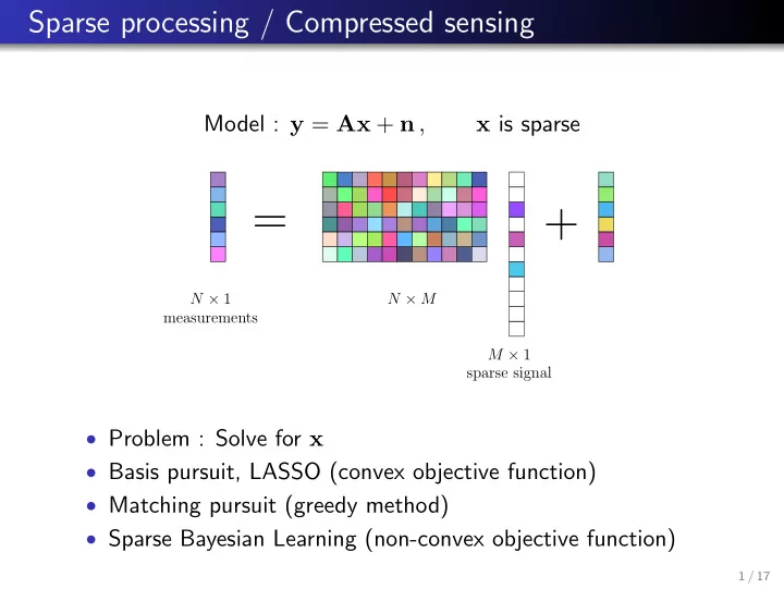
Sparse processing / Compressed sensing Model : y = Ax + n , x is sparse = + N 1 N M measurements M 1 sparse signal Problem : Solve for x Basis pursuit, LASSO (convex objective function) Matching pursuit (greedy method)
Sparse processing / Compressed sensing Model : y = Ax + n , x is sparse = + N × 1 N × M measurements M × 1 sparse signal • Problem : Solve for x • Basis pursuit, LASSO (convex objective function) • Matching pursuit (greedy method) • Sparse Bayesian Learning (non-convex objective function) 1 / 17
The unconstrained -LASSO- formulation Constrained formulation of the ` 1 -norm minimization problem: b x ` 1 ( � ) = arg min x 2 C N k x k 1 subject to k y − Ax k 2 ≤ � Unconstrained formulation in the form of least squares optimization with an ` 1 -norm regularizer: k y − Ax k 2 b x LASSO ( µ ) = arg min 2 + µ k x k 1 x 2 C N For every � exists a µ so that the two formulations are equivalent µ Regularization parameter : 2 / 17
Bayesian interpretation of unconstrained LASSO Bayes rule : Maximum a posteriori (MAP) estimate : 3 / 17
Bayesian interpretation of unconstrained LASSO Gaussian likelihood : Laplace Prior : MAP estimate : 4 / 17
Bayesian interpretation of unconstrained LASSO MAP estimate : 5 / 17
Prior and Posterior densities (Ex. Murphy) 6 / 17
Sparse Bayesian Learning (SBL) Model : y = Ax + n = + Prior : x ∼ N ( x ; 0 , Γ ) Γ = diag ( γ 1 , . . . , γ M ) N × 1 N × M measurements Likelihood : p ( y | x ) = N ( y ; Ax , σ 2 I N ) M × 1 sparse signal Evidence : SBL solution : M.E.Tipping, ”Sparse Bayesian learning and the relevance vector machine,” Journal of Machine Learning Research, June 2001. 7 / 17
SBL overview � � • SBL solution : ˆ log | Σ y | + y H Σ − 1 Γ = arg min y y Γ • SBL objective function is non-convex • Optimization solution is non-unique • Fixed point update using derivatives, works in practice • Γ = diag ( γ 1 , . . . , γ M ) || y H Σ − 1 y a m || 2 2 Update rule : γ new = γ old m m m Σ − 1 a H y a m Σ y = σ 2 I N + AΓA H • Multi snapshot extension : same Γ across snapshots 8 / 17
SBL overview • Posterior : x post = ΓA H Σ − 1 y y • At convergence, γ m → 0 for most γ m • Γ controls sparsity, E ( | x m | 2 ) = γ m iteration #0 150 . ( 3 ) 100 50 0 -90 -70 -50 -30 -10 10 30 50 70 90 Angle 3 ( ° ) • Different ways to show that SBL gives sparse output • Automatic determination of sparsity • Also provides noise estimate σ 2 9 / 17
Applications to acoustics - Beamforming • Beamforming • Direction of arrivals (DOAs) 10 / 17
SBL - Beamforming example • N = 20 sensors, uniform linear array • Discretize angle space: {− 90 : 1 : 90 } , M = 181 • Dictionary A : columns consist of steering vectors • K = 3 sources, DOAs, [ − 20 , − 15 , 75] ◦ , [12 , 22 , 20] dB • M ≫ N > K 20 CBF P (dB) 10 0 20 SBL . (dB) 10 0 -90 -70 -50 -30 -10 10 30 50 70 90 Angle 3 ( ° ) 11 / 17
SBL - Acoustic hydrophone data processing (from Kai) Ship of Opportunity Eigenrays CBF SBL 12 / 17
Problem with Degrees of Freedom • As the number of snapshots (=observations) increases, so does the number of unknown complex source amplitudes • PROBLEM: LASSO for multiple snapshots estimates the realizations of the random complex source amplitudes. • However, we would be satisfied if we just estimated their power γ m = E{ | x ml | 2 } • Note that γ m does not depend on snapshot index l . Thus SBL is much faster than LASSO for more snapshots. 13 / 17
Example CPU Time LASSO use CVX, CPU∝ L 2 SBL nearly independent on snapshots 200 1 b) c) SBL SBL 0.8 SBL1 DOA RMSE [ ° ] SBL1 CPU time (s) LASSO LASSO 10 0.6 0.4 1 0.2 0.1 0 1 10 100 1000 1 10 100 1000 Snapshots Snapshots 14 / 17
Matching Pursuit Model : y = Ax + n , x is sparse = + N × 1 N × M measurements M × 1 sparse signal • Greedy search method • Select column that is most aligned with the current residual 15 / 17
16 / 17
Amplitude Distribution � If the magnitudes of the non-zero elements in x 0 are highly scaled, then the canonical sparse recovery problem should be easier. x 0 x 0 � The (approximate) Jeffreys distribution produces For strongly scaled coefficients, Matching Pursuit (or sufficiently scaled coefficients such that best solution can Orthogonal MP) works better. It picks one coefficient at a time. always be easily computed. 17 / 17
Recommend
More recommend
Explore More Topics
Stay informed with curated content and fresh updates.
