Mutual Information Example - SSD 5 x 10 6 10 20 5 30 4 40 - PowerPoint PPT Presentation
Mutual Information Example - SSD 5 x 10 6 10 20 5 30 4 40 50 3 60 2 70 1 80 R I 90 10 20 30 40 50 60 70 Mutual Information Summary Statistical Tool for Dependence or of two variables Used as a tool for scoring
Mutual Information
Example - SSD 5 x 10 6 10 20 5 30 4 40 50 3 60 2 70 1 80 R I 90 10 20 30 40 50 60 70
Mutual Information Summary • Statistical Tool for Dependence or of two variables • Used as a tool for scoring similarity between data sets.
Sum of Squared Differences (SSD) 2 SSD , , , u v I x u y v R x y , x y E • SSD is optimal in the sense of ML when 1. Constant brightness assumption 2. Additive Gaussian noise
SSD Optimality For each pixel: 2 , , ~ 0 , I R x u y v x y N n P , , , I x u y v R x y u v 2 1 , , I R x u y v x y exp 2 2 2 n n
SSD Optimality – cont. For all pixels in area E: P , P , , , I R u v I x u y v R x y u v , x y A 2 1 , , I x u y v R x y logP , log exp I R u v 2 2 2 , x y A n n 2 , , I x u y v R x y const 2 2 , x y A n 2 max logP , min , , I R u v I x u y v R x y , u v A , x y
Example - SSD 5 x 10 6 10 20 5 30 4 40 50 3 60 2 70 1 80 R I 90 10 20 30 40 50 60 70
Normalized Cross-Correlation ~ ~ ~ , , I x u y v R x y I I I , x y A ~ NCC , u v ~ ~ R R R 2 2 , , I R x u y v x y , , x y A x y A • NCC is optimal in the sense of ML when 1. linear relationship between the images , , I x u y v R x y 2. Additive Gaussian noise
Example - NCC 5 x 10 0.8 7 10 10 6.5 0.6 20 20 6 30 30 0.4 5.5 40 40 5 0.2 50 50 4.5 0 4 60 60 -0.2 3.5 70 70 3 -0.4 80 80 R 2.5 90 90 -0.6 2 10 20 30 40 50 60 70 10 20 30 40 50 60 70 I’= 0.5I+30 true location NCC SSD
The Joint Histogram NCC Optimum SSD Optimum Y=aX+b Y=X Intensity of Transformed Target y Intensity of Reference x
Classic Use of Mutual Information in Registration of Data Sets ANGIO PET ATLAS MRI EEG CT
Cross Modality Registration Vo Uo T T = iter(T,Q) Q (Vo, Uo,T) How well can Vo Determine Uo? Do they have common information?
Information Theory - Entropy Shannon, “A mathematical theory of communication”, 1948 H=7.4635 1000 800 600 400 200 0 0 50 100 150 200 250 10000 log 9000 H=0 H A p a p a 8000 A A 7000 6000 a A 5000 4000 3000 2000 1000 0 0 50 100 150 200 250 Wide Distribution High entropy Uncertainty
Joint Entropy , , log , H A B p a b p a b AB AB a A b B p AB 7.399 , H A B 11.731 Higher Entropy more uncertainty Lower mutual information value
Information Theory – Mutual Information , , log , H A B p a b p a b AB AB a A b B A, B A B A, B I H H H I(A,B) A A | B H H B B | A H H H(B) H(A) In Two Variable we define Join Entropy in a similar way High Mutual information shared information How much entropy we lose because the parameters are couples
( , ) , I A B H A H B H A B A A A B B B matching A A B B non matching The closed the relationship is 1:1 between A/B the higher the MI
1000 800 600 400 200 0 0 50 100 150 200 250 T T' Poor Match Good Match
Comparing an image to itself results in the entropy of the image MI=5.53 It can not get any higher than that !!
ANGIO PET MRI CT MI is most useful in cross modalities registration where basic feature may not correspond in true values
Similar Regions / Symmetry Lines
Mutual Information Summary • Statistical Tool for Dependence or of two variables • Used as a tool for scoring similarity between data sets.
Recommend
More recommend
Explore More Topics
Stay informed with curated content and fresh updates.
