Multivariate models of inter-subject anatomical variability John - PowerPoint PPT Presentation
Introduction Geometric Variability Similarity Measures Real data Multivariate models of inter-subject anatomical variability John Ashburner Wellcome Trust Centre for Neuroimaging, UCL Institute of Neurology, 12 Queen Square, London WC1N
Introduction Geometric Variability Similarity Measures Real data Multivariate models of inter-subject anatomical variability John Ashburner Wellcome Trust Centre for Neuroimaging, UCL Institute of Neurology, 12 Queen Square, London WC1N 3BG, UK. John Ashburner Anatomical Features
Introduction Prediction Geometric Variability Binary Classification Similarity Measures Curse of dimensionality Real data “ The only relevant test of the validity of a hypothesis is comparison of prediction with experience .” Milton Friedman John Ashburner Anatomical Features
Introduction Prediction Geometric Variability Binary Classification Similarity Measures Curse of dimensionality Real data Choosing models/hypotheses/theories MacKay, DJC. “Bayesian interpolation.” Neural computation 4, no. 3 (1992): 415-447. John Ashburner Anatomical Features
Introduction Prediction Geometric Variability Binary Classification Similarity Measures Curse of dimensionality Real data Evidence-based Science ...also just known as “science”. Researchers claim to find differences between groups. Do those findings actually discriminate? How can we most accurately diagnose a disorder from image data? Pharma wants biomarkers. How do we most effectively identify them? There are lots of potential imaging biomarkers. Which are most (cost) effective? Pattern recognition provides a framework to compare data (or preprocessing strategy) to determine the most accurate approach. John Ashburner Anatomical Features
Introduction Prediction Geometric Variability Binary Classification Similarity Measures Curse of dimensionality Real data Biological variability is multivariate John Ashburner Anatomical Features
Introduction Prediction Geometric Variability Binary Classification Similarity Measures Curse of dimensionality Real data A generative classification approach p(x,y=0) = p(x|y=0) p(y=0) p(x,y=1) = p(x|y=1) p(y=1) −1 −1 −2 −2 −3 −3 Feature 2 Feature 2 −4 −4 −5 −5 −6 −6 −7 −7 0 2 4 0 2 4 Feature 1 Feature 1 p(x) = p(x,y=0) + p(x,y=1) p(y=0|x) = p(x,y=0)/p(x) −1 −1 −2 −2 −3 −3 Feature 2 Feature 2 −4 −4 −5 −5 −6 −6 −7 −7 0 2 4 0 2 4 Feature 1 Feature 1 John Ashburner Anatomical Features
Introduction Prediction Geometric Variability Binary Classification Similarity Measures Curse of dimensionality Real data Discriminative classification approaches Ground truth FLDA −1 −1 −2 −2 −3 −3 Feature 2 Feature 2 −4 −4 −5 −5 −6 −6 −7 −7 0 2 4 0 2 4 Feature 1 Feature 1 SVC Simple Logistic Regression −1 −1 −2 −2 −3 −3 Feature 2 Feature 2 −4 −4 −5 −5 −6 −6 −7 −7 0 2 4 0 2 4 Feature 1 Feature 1 John Ashburner Anatomical Features
Introduction Prediction Geometric Variability Binary Classification Similarity Measures Curse of dimensionality Real data Bayesian classification Simple Logistic Regression Hyperplane Uncertainty −1 −1 −2 −2 −3 −3 Feature 2 Feature 2 −4 −4 −5 −5 −6 −6 −7 −7 0 2 4 0 2 4 Feature 1 Feature 1 Bayesian Logistic Regression Bayesian Logistic Regression −1 −1 −2 −2 −3 −3 Feature 2 Feature 2 −4 −4 −5 −5 −6 −6 −7 −7 0 2 4 0 2 4 Feature 1 Feature 1 John Ashburner Anatomical Features
Introduction Prediction Geometric Variability Binary Classification Similarity Measures Curse of dimensionality Real data Why Bayesian? To deal with different priors. Consider a method with 90% sensitivity and specificity. Consider using this to screen for a disease afflicting 1% of the population. On average, out of 100 people there would be 10 wrongly assigned to the disease group. A positive diagnosis suggests only about a 10% chance of having the disease. P (Pred+ | Disease) P (Disease) P (Disease | Pred+) = P (Pred+ | Disease) P (Disease)+ P (Pred+ | Healthy) P (Healthy) Sensitivity × P (Disease) = Sensitivity × P (Disease)+(1 − Specificity ) × P (Healthy) Better decision-making by accounting for utility functions. John Ashburner Anatomical Features
Introduction Prediction Geometric Variability Binary Classification Similarity Measures Curse of dimensionality Real data Curse of dimensionality Large p , small n . John Ashburner Anatomical Features
Introduction Prediction Geometric Variability Binary Classification Similarity Measures Curse of dimensionality Real data Nearest-neighbour classification 2 Not nice 1 smooth separations. Feature 2 Lots of sharp 0 corners. May be −1 improved with K-nearest −2 neighbours . −3 −2 −1 0 1 2 Feature 1 John Ashburner Anatomical Features
Introduction Prediction Geometric Variability Binary Classification Similarity Measures Curse of dimensionality Real data Rule-based approaches ((x<0.3) & (y<2)) | ((x<0.75) & (y<1.25)) | (y<0.4) 4 3 Not nice smooth 2 y separations. Lots of sharp 1 corners. 0 0 1 2 3 4 x John Ashburner Anatomical Features
Introduction Prediction Geometric Variability Binary Classification Similarity Measures Curse of dimensionality Real data Corners matter in high-dimensions John Ashburner Anatomical Features
Introduction Prediction Geometric Variability Binary Classification Similarity Measures Curse of dimensionality Real data Corners matter in high-dimensions 1 0.9 0.8 Circle area = π r 2 0.7 Volume of hyper−sphere (r=1/2) 0.6 Sphere volume = 4/3 π r 3 0.5 0.4 0.3 0.2 0.1 0 0 2 4 6 8 10 12 14 16 18 20 Number of dimensions John Ashburner Anatomical Features
Introduction Prediction Geometric Variability Binary Classification Similarity Measures Curse of dimensionality Real data Dimensionality � = number of voxels Little evidence to suggest that most voxel-based feature selection methods help. Little or no increase in predictive accuracy. Commonly perceived as being more “interpretable”. Prior knowledge derived from independent data is the most reliable way to improve accuracy. e.g. search the literature for clues about which regions to weight more heavily. Cuingnet, R´ emi, Emilie Gerardin, J´ erˆ ome Tessieras, Guillaume Auzias, St´ ephane Leh´ ericy, Marie-Odile Habert, Marie Chupin, Habib Benali, and Olivier Colliot. “Automatic classification of patients with Alzheimer’s disease from structural MRI: a comparison of ten methods using the ADNI database.” Neuroimage 56, no. 2 (2011): 766-781. Chu, Carlton, Ai-Ling Hsu, Kun-Hsien Chou, Peter Bandettini, and ChingPo Lin. “Does feature selection improve classification accuracy? Impact of sample size and feature selection on classification using anatomical magnetic resonance images.” Neuroimage 60, no. 1 (2012): 59-70. See winning strategies in http://www.ebc.pitt.edu/PBAIC.html John Ashburner Anatomical Features
Introduction Prediction Geometric Variability Binary Classification Similarity Measures Curse of dimensionality Real data Linear versus Nonlinear methods Raw Data Linear methods are more interpretable. 10 Nonlinear methods usually increase 8 Feature 2 6 dimensionality. 4 Better to preprocess to obtain features 2 that behave more linearly. 2 4 6 8 10 Feature 1 Body Mass Index (linear plot) Body Mass Index (log−log plot) 2 2 BMI=18.5 BMI=18.5 Log−Transformed BMI=25 BMI=25 1.9 1 BMI=30 BMI=30 1.9 10 1.8 1.8 Height (m) Height (m) 0 1.7 10 Feature 2 1.7 1.6 1.6 −1 10 1.5 1.5 1.4 1.4 40 50 60 70 80 90 100 110 120 130 140 150 160 40 50 60 70 80 90 100 120 140 160 0 Weight (kg) Weight (kg) 10 Feature 1 John Ashburner Anatomical Features
Introduction Geometric Variability Manifolds Similarity Measures Principal Components Real data Transformed images fall on manifolds Rotating an image leads to points on a 1D manifold. 0.7 0.6 0.5 0.4 0.3 0.2 0.1 0 0 0.2 0.4 0.6 Rigid-body motion leads to a 6-dimensional manifold (not shown). John Ashburner Anatomical Features
Introduction Geometric Variability Manifolds Similarity Measures Principal Components Real data Local linearisation through smoothing 800 700 600 500 Spatial smoothing 400 300 can make the 200 manifolds more 100 linear with respect 0 0 200 400 600 800 to small 400 misregistrations. 350 Some information is 300 250 inevitably lost. 200 150 100 50 0 0 100 200 300 400 John Ashburner Anatomical Features
Introduction Geometric Variability Manifolds Similarity Measures Principal Components Real data One mode of geometric variability Simulated images Principal components A suitable model would reduce these data to a single dimension. John Ashburner Anatomical Features
Introduction Geometric Variability Manifolds Similarity Measures Principal Components Real data Two modes of geometric variability Simulated images Principal components A suitable model would reduce these data to two dimensions. John Ashburner Anatomical Features
Recommend
More recommend
Explore More Topics
Stay informed with curated content and fresh updates.
