Multivariate comonotonicity, stochastic orders and risk measures - PDF document
Multivariate comonotonicity, stochastic orders and risk measures Alfred Galichon (Ecole polytechnique) Brussels, May 25, 2012 Based on collaborations with: A. Charpentier (Rennes) G. Carlier (Dauphine) R.-A. Dana (Dauphine)
Multivariate comonotonicity, stochastic orders and risk measures Alfred Galichon (Ecole polytechnique) Brussels, May 25, 2012 Based on collaborations with: – A. Charpentier (Rennes) – G. Carlier (Dauphine) – R.-A. Dana (Dauphine) – I. Ekeland (Dauphine) – M. Henry (Montréal)
This talk will draw on four papers: [CDG]. “Pareto e¢ciency for the concave order and mul- tivariate comonotonicity”. Guillaume Carlier, Alfred Gali- chon and Rose-Anne Dana. Journal of Economic Theory, 2012 . [CGH] “"Local Utility and Multivariate Risk Aversion”. Arthur Charpentier, Alfred Galichon and Marc Henry. Mimeo. [GH] “Dual Theory of Choice under Multivariate Risks”. Alfred Galichon and Marc Henry. Journal of Economic Theory, forthcoming . [EGH] “Comonotonic measures of multivariate risks”. Ivar Ekeland, Alfred Galichon and Marc Henry. Mathematical Finance, 2011 .
Introduction Comonotonicity is a central tool in decision theory, insur- ance and …nance. Two random variables are « comonotone » when they are maximally correlated, i.e. when there is a nondecreasing map from one to another. Applications include risk mea- sures, e¢cient risk-sharing, optimal insurance contracts, etc. Unfortunately, no straightforward extension to the multi- variate case (i.e. when there are several numeraires). The goal of this presentation is to investigate what hap- pens in the multivariate case, when there are several di- mension of risk. Applications will be given to: – Risk measures, and their aggregation – E¢cient risk-sharing – Stochastic ordering.
1 Comonotonicity and its general- ization 1.1 One-dimensional case Two random variables X and Y are comonotone if there exists a r.v. Z and nondecreasing maps T X and T Y such that X = T X ( Z ) and Y = T Y ( Z ) : For example, if X and Y are sampled from empirical distributions, X ( ! i ) = x i and Y ( ! i ) = y i , i = 1 ; :::; n where x 1 � ::: � x n and y 1 � ::: � y n then X and Y are comonotonic.
By the rearrangement inequality (Hardy-Littlewood), n n X X max x i y � ( i ) = x i y i : � permutation i =1 i =1 More generally, X and Y are comonotonic if and only if h i X ~ E = E [ XY ] : max Y ~ Y = d Y
Example . Consider ! ! 1 ! 2 P ( ! ) 1 = 2 1 = 2 X ( ! ) +1 � 1 Y ( ! ) +2 � 2 ~ Y ( ! ) � 2 +2 X and Y are comonotone. ~ Y has the same distribution as Y but is not comonotone with X . One has h i X ~ E [ XY ] = 2 > � 2 = E Y :
Hardy-Littlewood inequality . The probability space is now [0 ; 1] . Assume U ( t ) = � ( t ) , where � is nonde- creasing. Let P a probability distribution, and let X ( t ) = F � 1 P ( t ) : For ~ X : [0 ; 1] ! R a r.v. such that ~ X � P , one has Z 1 h ~ i 0 � ( t ) F � 1 E [ XU ] = P ( t ) dt � E XU : Thus, letting Z 1 n o 0 � ( t ) F � 1 E [ ~ XU ] ; ~ % ( X ) = X ( t ) dt = max X = d X n o E [ X ~ U ] ; ~ = max U = d U :
A geometric characterization. Let � be an absolutely continuous distribution; two random variables X and Y are comonotone if for some random variable U � � , we have n o E [ X ~ U ] ; ~ U 2 argmax ~ U � � , and U n o E [ Y ~ U ] ; ~ U 2 argmax ~ U � � : U Geometrically, this means that X and Y have the same projection of the equidistribution class of � =set of r.v. with distribution � .
1.2 Multivariate generalization Problem: what can be done for risks which are multidi- mensional, and which are not perfect substitutes? Why? risk usually has several dimension (price/liquidity; multicurrency portfolio; environmental/…nancial risk, etc). Concepts used in the univariate case do not directly ex- tend to the multivariate case.
The variational characterization given above will be the basis for the generalized notion of comonotonicity given in [EGH]. De…nition ( � -comonotonicity). Let � be an atomless probability measure on R d . Two random vectors X and Y in L 2 d are called � -comonotonic if for some random vector U � � , we have n o E [ X � ~ U ] ; ~ , and U 2 argmax ~ U � � U n o E [ Y � ~ U ] ; ~ U argmax ~ U � � 2 U equivalentely: X and Y are � -comonotonic if there exists two convex functions V 1 and V 2 and a random variable U � � such that X = r V 1 ( U ) Y = r V 2 ( U ) : Note that in dimension 1, this de…nition is consistent with the previous one.
Monge-Kantorovich problem and Brenier theorem Let � and P be two probability measures on R d with second moments, such that � is absolutely continuous. Then sup E [ h U; X i ] U � �;X � P where the supremum is over all the couplings of � and P if attained for a coupling such that one has X = r V ( U ) almost surely, where V is a convex function R d ! R which happens to be the solution of the dual Kantorovich problem Z Z inf V ( u ) d� ( u ) + W ( x ) dP ( x ) : V ( u )+ W ( x ) �h x;u i Call Q P ( u ) = r V ( u ) the � -quantile of distribution P .
Comonotonicity and transitivity . Puccetti and Scarsini (2010) propose the following de…n- ition of comonotonicity, called c -comonotonicity: X and Y are c -comonotone if and only if n o E [ X � ~ Y ] ; ~ Y 2 argmax ~ Y � Y Y or, equivalently, i¤ there exists a convex function u such that Y 2 @u ( X ) that is, whenever u is di¤erentiabe at X , Y = r u ( X ) : However, this de…nition is not transitive: if X and Y are c -comonotone and Y and Z are c -comonotone, and if the distributions of X , Y and Z are absolutely continuous, then X and Z are not necessarily c -comonotome. This transivity (true in dimension one) may however be seen as desirable.
In the case of � -comonotonicity, transitivity holds: if X and Y are � -comonotone and Y and Z are � -comonotone, and if the distributions of X , Y and Z are absolutely con- tinuous, then X and Z are � -comonotome. Indeed, express � -comonotonicity of X and Y : for some U � � , X = r V 1 ( U ) Y = r V 2 ( U ) and by � -comonotonicity of Y and Z , for some ~ U � � , � ~ � Y = r V 2 U � ~ � Z = r V 3 U this implies ~ U = U , and therefore X and Z are � - comonotone.
Importance of � . In dimension one, one recovers the classical notion of comotonicity regardless of the choice of � . However, in dimension greater than one, the comonotonic- ity relation crucially depends on the baseline distribution � , unlike in dimension one. The following lemma from [EGH] makes this precise: Lemma. Let � and � be atomless probability measures on R d . Then: - In dimension d = 1 , � -comonotonicity always implies � -comonotonicity. - In dimension d � 2 , � -comonotonicity implies � -comonotonicity if and only if � = T # � for some location-scale transform T ( u ) = �u + u 0 where � > 0 and u 0 2 R d . In other words, comonotonicity is an invariant of the location- scale family classes.
2 Applications to risk measures 2.1 Coherent, regular risk measures (uni- variate case) Following Artzner, Delbaen, Eber, and Heath, recall the classical risk measures axioms: Recall axioms: De…nition. A functional % : L 2 d ! R is called a coherent risk measure if it satis…es the following properties: - Monotonicity (MON): X � Y ) % ( X ) � % ( Y ) - Translation invariance (TI): % ( X + m ) = % ( X )+ m% (1) - Convexity (CO): % ( �X + (1 � � ) Y ) � �% ( X ) + (1 � � ) % ( Y ) for all � 2 (0 ; 1) . - Positive homogeneity (PH): % ( �X ) = �% ( X ) for all � � 0 .
De…nition. % : L 2 ! R is called a regular risk measure if it satis…es: - Law invariance (LI): % ( X ) = % ( ~ X ) when X � ~ X . - Comonotonic additivity (CA): % ( X + Y ) = % ( X ) + % ( Y ) when X; Y are comonotonic, i.e. weakly increasing transformation of a third randon variable: X = � 1 ( U ) and Y = � 2 ( U ) a.s. for � 1 and � 2 nondecreasing. Result (Kusuoka, 2001). A coherent risk measure % is regular if and only if for some increasing and nonnegative function � on [0 ; 1] , we have Z 1 0 � ( t ) F � 1 % ( X ) := X ( t ) dt; where F X denotes the cumulative distribution functions of the random variable X (thus Q X ( t ) = F � 1 X ( t ) is the associated quantile). % is called a Spectral risk measure . For reasons explained later, also called Maximal correlation risk measure .
Leading example: Expected shortfall (also called Con- 1 ditional VaR or TailVaR ): � ( t ) = 1 � � 1 f t � � g : Then Z 1 1 � F � 1 % ( X ) := X ( t ) dt: 1 � �
Kusuoka’s result, intuition. � � F � 1 � Law invariance ) % ( X ) = � X � Comonotone additivity+positive homogeneity ) � is linear w.r.t. F � 1 X : � � R 1 F � 1 0 � ( t ) F � 1 � = X ( t ) dt . X � Monotonicity ) � is nonnegative � Subadditivity ) � is increasing Unfortunately, this setting does not extend readily to mul- tivariate risks. We shall need to reformulate our axioms in a way that will lend itself to easier multivariate extension.
Recommend
More recommend
Explore More Topics
Stay informed with curated content and fresh updates.
