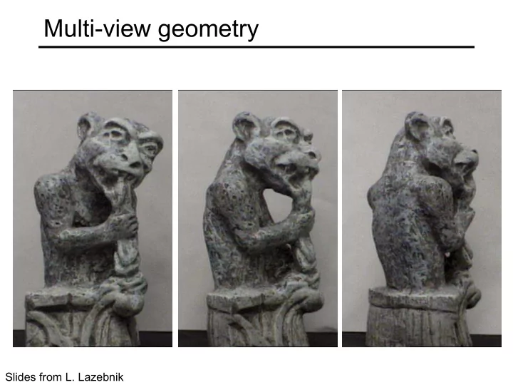
Multi-view geometry Slides from L. Lazebnik Structure from motion - PowerPoint PPT Presentation

Multi-view geometry Slides from L. Lazebnik

Structure from motion Camera 1 Camera 3 Camera 2 R 1 ,t 1 R 3 ,t 3 R 2 ,t 2 Figure credit: Noah Snavely

Structure from motion ? Camera 1 Camera 3 Camera 2 R 1 ,t 1 R 3 ,t 3 R 2 ,t 2 • Structure: Given known cameras and projections of the same 3D point in two or more images, compute the 3D coordinates of that point

Structure from motion Camera 1 ? Camera 3 ? Camera 2 R 1 ,t 1 ? R 3 ,t 3 R 2 ,t 2 • Motion: Given a set of known 3D points seen by a camera, compute the camera parameters

Structure from motion Camera 1 ? Camera 2 R 1 ,t 1 ? R 2 ,t 2 • Bootstrapping the process: Given a set of 2D point correspondences in two images , compute the camera parameters

Two-view geometry

Epipolar geometry X x x’ • Baseline – line connecting the two camera centers • Epipolar Plane – plane containing baseline (1D family) • Epipoles = intersections of baseline with image planes = projections of the other camera center = vanishing points of the motion direction

Epipolar geometry X x x’ • Baseline – line connecting the two camera centers • Epipolar Plane – plane containing baseline (1D family) • Epipoles = intersections of baseline with image planes = projections of the other camera center = vanishing points of the motion direction • Epipolar Lines - intersections of epipolar plane with image planes (always come in corresponding pairs)

Example 1 • Converging cameras

Example 2 • Motion parallel to the image plane

Example 3

Example 3 • Motion is perpendicular to the image plane • Epipole is the “focus of expansion” and the principal point

Motion perpendicular to image plane http://vimeo.com/48425421

Epipolar constraint X x x’ • If we observe a point x in one image, where can the corresponding point x’ be in the other image?

Epipolar constraint X X X x x’ x’ x’ • Potential matches for x have to lie on the corresponding epipolar line l ’ . • Potential matches for x ’ have to lie on the corresponding epipolar line l .

Epipolar constraint example

Epipolar constraint: Calibrated case X x x’

Epipolar constraint: Calibrated case X x x’ • Intrinsic and extrinsic parameters of the cameras are known, world coordinate system is set to that of the first camera • Then the projection matrices are given by K [ I | 0] and K ’[ R | t ] • We can multiply the projection matrices (and the image points) by the inverse of the calibration matrices to get normalized image coordinates: ¢ ¢ ¢ = - = = - = 1 1 x K x [ I 0] X, x K x [ R t ] X norm pixel norm pixel

Epipolar constraint: Calibrated case Derivation X x x’

Epipolar constraint: Calibrated case Derivation X x x’

Epipolar constraint: Calibrated case Simplification X = ( x, 1) T æ ö æ ö x x [ ] [ ] ç ÷ ç ÷ I 0 R t ç ÷ ç ÷ 1 1 è ø è ø x x’ = Rx+t 𝑦′ 𝑆𝑦 + 𝑢 𝑢 t R é ù - é ù Recall: 0 a a b z y x ê ú ê ú ´ = - = a b a 0 a b [ a ] b ê ú ê ú ´ z x y ê ú ê ú - a a 0 b ë û ë û y x z The vectors 𝑆𝑦 + 𝑢 , 𝑢 , and 𝑦′ are coplanar

Epipolar constraint: Calibrated case Simplification X = ( x, 1) T æ ö æ ö x x [ ] [ ] ç ÷ ç ÷ I 0 R t ç ÷ ç ÷ 1 1 è ø è ø x x’ = Rx+t 𝑦′ 𝑆𝑦 + 𝑢 𝑢 t 𝑦 ! . 𝑢× 𝑆𝑦 + 𝑢 = 0 R 𝑦 ! . 𝑢×𝑆𝑦 + 𝑢×𝑢 = 0 é ù - é ù Recall: 0 a a b z y x ê ú 𝑦 ! . 𝑢×𝑆𝑦 = 0 𝑦 !# 𝐹𝑦 = 0 ê ú ´ = - = a b a 0 a b [ a ] b ê ú ê ú ´ z x y 𝑦 ! . 𝑢 × 𝑆𝑦 = 0 ê ú ê ú - a a 0 b ë û ë û y x z The vectors 𝑆𝑦 + 𝑢 , 𝑢 , and 𝑦′ are coplanar

Epipolar constraint: Calibrated case X = ( x, 1) T æ ö æ ö x x [ ] [ ] ç ÷ ç ÷ I 0 R t ç ÷ ç ÷ 1 1 è ø è ø x x’ = Rx+t 𝑦′ 𝑆𝑦 + 𝑢 𝑢 ¢ × ´ = x T E x = 0 x T [ t × ] Rx = 0 x [ t ( R x ) ] 0 ! ! Essential Matrix (Longuet-Higgins, 1981) The vectors 𝑆𝑦 + 𝑢 , 𝑢 , and 𝑦′ are coplanar

Epipolar constraint: Calibrated case X x x’ x T E x = 0 ! • E x is the epipolar line associated with x ( l ' = E x ) • Recall: a line is given by ax + by + c = 0 or é ù é ù a x ê ú ê ú = = = T l x 0 where l b , x y ê ú ê ú ê ú ê ú c 1 ë û ë û

Epipolar constraint: Calibrated case X x x’ x T E x = 0 ! • E x is the epipolar line associated with x ( l ' = E x ) • E T x ' is the epipolar line associated with x' ( l = E T x ' ) • E e = 0 and E T e ' = 0 • E is singular (rank two) • E has five degrees of freedom

Epipolar constraint: Uncalibrated case X x x’ • The calibration matrices K and K ’ of the two cameras are unknown • We can write the epipolar constraint in terms of unknown normalized coordinates:

Epipolar constraint: Uncalibrated case X x x’ • The calibration matrices K and K ’ of the two cameras are unknown • We can write the epipolar constraint in terms of unknown normalized coordinates: ¢ ¢ ¢ - - = = ¢ ˆ 1 ˆ 1 = x T x K x , x K x ˆ ˆ E x 0

Epipolar constraint: Uncalibrated case X x x’ ¢ ¢ ¢ - - = = = x T ˆ ˆ T T 1 E x 0 x F x 0 with F K E K - = 1 ˆ x K x Fundamental Matrix ¢ ¢ ¢ - = 1 ˆ x K x (Faugeras and Luong, 1992)

Epipolar constraint: Uncalibrated case X x x’ ¢ ¢ ¢ - - = = = x T ˆ ˆ T T 1 E x 0 x F x 0 with F K E K • F x is the epipolar line associated with x ( l ' = F x ) • F T x ' is the epipolar line associated with x' ( l = F T x ' ) • F e = 0 and F T e ' = 0 • F is singular (rank two) • F has seven degrees of freedom

Estimating the fundamental matrix

The eight-point algorithm ¢ ¢ ¢ = = T x ( u , v , 1 ) , x ( u , v , 1 )

The eight-point algorithm ¢ ¢ ¢ é ù = = f T x ( u , v , 1 ) , x ( u , v , 1 ) 11 ê ú f ê ú 12 ê ú f 13 ê ú é f f f ù é u ù f ê ú 11 12 13 21 ê ú ê ú [ ] [ ] ¢ ¢ = ê ú ¢ ¢ ¢ ¢ ¢ ¢ u v 1 f f f v 0 = u u u v u v u v v v u v 1 f 0 ê ú ê ú 21 22 23 22 ê ú ê ú ê ú f f f f 1 ê ú ë û ë û Solve homogeneous 23 31 32 33 ê ú f ê ú 31 linear system using ê f ú 32 eight or more matches ê ú f ë û 33 Enforce rank-2 constraint (take SVD of F and throw out the smallest singular value)

Problem with eight-point algorithm é ù f 11 ê ú f ê ú 12 ê ú f 13 ê ú f [ ] ê ú ¢ ¢ ¢ ¢ ¢ ¢ 21 = - u u u v u v u v v v u v 1 ê ú f 22 ê ú f ê ú 23 ê ú f ê ú 31 ê ú f ë û 32

Problem with eight-point algorithm é ù f 11 ê ú f ê ú 12 ê ú f 13 ê ú f [ ] ê ú ¢ ¢ ¢ ¢ ¢ ¢ 21 = - u u u v u v u v v v u v 1 ê ú f 22 ê ú f ê ú 23 ê ú f ê ú 31 ê ú f ë û Poor numerical conditioning 32 Can be fixed by rescaling the data

The normalized eight-point algorithm (Hartley, 1995) • Center the image data at the origin, and scale it so the mean squared distance between the origin and the data points is 2 pixels • Use the eight-point algorithm to compute F from the normalized points • Enforce the rank-2 constraint (for example, take SVD of F and throw out the smallest singular value) • Transform fundamental matrix back to original units: if T and T ’ are the normalizing transformations in the two images, than the fundamental matrix in original coordinates is T ’ T F T

Seven-point algorithm • Set up least squares system with seven pairs of correspondences and solve for null space (two vectors) using SVD • Solve for linear combination of null space vectors that satisfies det(F)=0 Source: D. Hoiem

Nonlinear estimation • Linear estimation minimizes the sum of squared algebraic distances between points x ’ i and epipolar lines F x i (or points x i and epipolar lines F T x ’ i ): N ∑ x i T F x i ) 2 ( ! i = 1 • Nonlinear approach: minimize sum of squared geometric distances N x i , F x i ) + d 2 ( x i , F T ! ∑ " x i ) $ d 2 ( ! # % i = 1 x i x i ! Fx i F T ! x i

Comparison of estimation algorithms 8-point Normalized 8-point Nonlinear least squares Av. Dist. 1 2.33 pixels 0.92 pixel 0.86 pixel Av. Dist. 2 2.18 pixels 0.85 pixel 0.80 pixel

The Fundamental Matrix Song http://danielwedge.com/fmatrix/

From epipolar geometry to camera calibration • Estimating the fundamental matrix is known as “weak calibration” • If we know the calibration matrices of the two cameras, we can estimate the essential matrix: E = K ’ T FK • The essential matrix gives us the relative rotation and translation between the cameras, or their extrinsic parameters • Alternatively, if the calibration matrices are known, the five-point algorithm can be used to estimate relative camera pose