Epipolar Geometry EECS 442 David Fouhey Fall 2019, University of - PowerPoint PPT Presentation
Epipolar Geometry EECS 442 David Fouhey Fall 2019, University of Michigan http://web.eecs.umich.edu/~fouhey/teaching/EECS442_F19/ Multi-view geometry Image Credit: S. Lazebnik Multi-view geometry problems Recovering structure: ? Given
Epipolar Geometry EECS 442 – David Fouhey Fall 2019, University of Michigan http://web.eecs.umich.edu/~fouhey/teaching/EECS442_F19/
Multi-view geometry Image Credit: S. Lazebnik
Multi-view geometry problems Recovering structure: ? Given cameras and correspondences, find 3D. Camera 1 Camera 3 Camera 2 R 1 ,t 1 R 3 ,t 3 R 2 ,t 2 Slide credit: Noah Snavely
Multi-view geometry problems Stereo/Epipolar Geomery: Given 2 cameras and find where a point could be Camera 1 Camera 3 Camera 2 R 1 ,t 1 R 3 ,t 3 R 2 ,t 2 Slide credit: Noah Snavely
Multi-view geometry problems Motion: Figure out R, t for a set of cameras given correspondences ? Camera 1 Camera 3 ? Camera 2 ? R 1 ,t 1 R 3 ,t 3 R 2 ,t 2 Slide credit: Noah Snavely
Two-view geometry Image Credit: Hartley & Zisserman
Camera Geometry Reminder X (3D point) K -1 p (Ray) 4 h. coordinates 3 h. coordinates p (2D point) 0 3 h. coordinates Pretending image p (2D point) plane is in front 3 h. coordinates Actual location Have camera with pinhole at origin 0
Epipolar Geometry o o' Suppose we have two cameras at origins o, o’ Baseline is the line connecting the origins
Epipolar Geometry X p p' o o' Now add a point X , which projects to p and p’
Epipolar Geometry X p p' o o' The plane formed by X, o, and o’ is called the epipolar plane There is a family of planes per o, o’
Epipolar Geometry X p p' o o' e e' • Epipoles e, e’ are where the baseline intersects the image planes • Projection of other camera in the image plane
The Epipole Photo by Frank Dellaert
Epipolar Geometry X p p' o o' e e' • Epipolar lines go between the epipoles and the projections of the points. • Intersection of epipolar plane with image plane
Example: Converging Cameras p p' o o' e e' Epipoles finite, maybe in image; epipolar lines converge
Example: Converging Cameras p p' o o' e e' Epipolar lines come in pairs: given a point p, we can construct the epipolar line for p’.
Example 1: Converging Cameras Image Credit: Hartley & Zisserman
Example: Parallel to Image Plane Suppose the cameras are both facing outwards. Where are the epipoles (proj. of other camera)?
Example: Parallel to Image Plane p' p e' e Epipoles infinitely far away, epipolar lines parallel
Example: Parallel to Image Plane Image Credit: Hartley & Zisserman
Example: Forward Motion Image Credit: Hartley & Zisserman
Example: Forward Motion Image Credit: Hartley & Zisserman
Example: Forward Motion Epipole is focus of expansion / principal point of the camera. Epipolar lines go out from principal point
Motion perpendicular to image plane http://vimeo.com/48425421
So?
Epipolar Geometry p o o' e e' • Suppose we don’t know X and just have p • Can construct the epipolar line in the other image
Epipolar Geometry p o o' e e' • Suppose we don’t know X and just have p • Corresponding p’ is on corresponding epipolar line
Epipolar Geometry p' o o' e e' • Suppose we don’t know X and just have p’ • Corresponding p is on corresponding epipolar line
Epipolar Geometry • If I want to do stereo, I want to find a corresponding pixel for each pixel in the image: • Naïve search: • For each pixel, search every other pixel • With epipolar geometry: • For each pixel, search along each line (1D search)
Epipolar constraint example Slide Credit: S. Lazebnik
Epipolar Constraint: One Note • If you look around for other reading, you’ll find derivations with p, p’ flipped and constraints derived in a flipped way • It all works the same
Epipolar Constraint: Calibrated Case X p p' o o' 𝑺, 𝒖 • If we know intrinsic and extrinsic parameters, set coordinate system to first camera Projection matrices: 𝐐 1 = 𝑳 𝑱, 𝟏 and 𝑸 𝟑 = 𝑳 ′ 𝑺, 𝒖 • • What are: 𝑳 ′−𝟐 𝒒′ 𝑳 −𝟐 𝒒 𝑸 𝟐 𝒀 𝑸 𝟑 𝒀
Epipolar Constraint: Calibrated Case X 𝒒′ = 𝑳′ −𝟐 𝒒′ 𝒒 = 𝑳 −𝟐 𝒒 ෝ p p' o o' 𝑺, 𝒖 𝒒 ′ = 𝑳 ′−𝟐 𝒒′ are 𝒒 = 𝑳 −𝟐 𝒒 and • Given calibration, ෝ “normalized coordinates” Note that • 𝑞′ is actually translated and rotated
Epipolar Constraint: Calibrated Case X 𝒒′ = 𝑳′ −𝟐 𝒒′ 𝒒 = 𝑳 −𝟐 𝒒 ෝ p p' o o' 𝑺, 𝒖 𝒒 , 𝒖 , 𝑺 • The following are all co-planar: ෝ 𝒒′ (can ignore translation for co-planarity here) • One way to check co-planarity (triple product): 𝒒 𝑼 𝒖 × 𝑺ෝ ෝ 𝒒 = 0
Epipolar Constraint: Calibrated Case X 𝒒′ = 𝑳′ −𝟐 𝒒′ 𝒒 = 𝑳 −𝟐 𝒒 ෝ p p' o o' 𝑺, 𝒖 [𝑢 𝑦 ] 0 −𝑢 3 𝑢 2 𝒒 𝑼 𝒖 × 𝑺ෝ 𝑺 𝒒 𝑼 𝑢 3 0 −𝑢 1 ෝ 𝒒′ = 0 ෝ 𝒒′ = 0 −𝑢 2 𝑢 1 0 Want something like x T My =0. What’s M?
Epipolar Constraint: Calibrated Case X 𝒒′ = 𝑳′ −𝟐 𝒒′ 𝒒 = 𝑳 −𝟐 𝒒 ෝ p p' o o' 𝑺, 𝒖 Essential matrix (Longuet-Higgins, 1981): 𝑭 = 𝒖 𝒚 𝑺 If you have a normalized point ෝ 𝒒 , its correspondence ෝ 𝒒′ 𝒒 𝑼 𝑭 must satisfy ෝ 𝒒′ = 0
Essential Essential Matrix Facts X 𝒒 = 𝑳 −𝟐 𝒒 p 𝒒′ = 𝑳′ −𝟐 𝒒′ ෝ p' o o' 𝒒 𝑼 𝑭 • Suppose we know E and ෝ 𝒒′ = 0 . What is the set 𝒒 ′ = 𝟏} ? {𝒚: 𝒚 𝑼 𝑭 • 𝒒 gives equation of the epipolar line (in ax+by+c=0 𝑭ෝ form) in image for o. What’s 𝑭 𝑼 ෝ • 𝒒 ?
Essential Essential Matrix Facts X 𝒒 = 𝑳 −𝟐 𝒒 p 𝒒′ = 𝑳′ −𝟐 𝒒′ ෝ p' e e' o o' 𝒇 ′ = 0 and 𝑭 𝑼 ො • 𝑭 𝒇 = 0 (epipoles are the nullspace of E – note all epipolar lines pass through epipoles) • Degrees of freedom (Recall 𝑭 = 𝒖 𝒚 𝑺 )? • 5 – 3 (R)+ 3 (t) – 1 due to scale ambiguity • E is singular (rank 2); it has two non-zero and identical singular values
Essential Essential Matrix Facts X 𝒒 = 𝑳 −𝟐 𝒒 p 𝒒′ = 𝑳′ −𝟐 𝒒′ ෝ p' e e' o o' • One nice thing: if I estimate E from two images (more on this later), it’s unique up to easy symmetries
What if we don’t know K? X 𝒒 = 𝑳 −𝟐 𝒒 p 𝒒′ = 𝑳′ −𝟐 𝒒′ ෝ p' o o' 𝒒 ′ = 0 𝒒 = 𝑳 −𝟐 𝒒, 𝒒 𝑼 𝑭ෝ Have: 𝒒′ = 𝑳′ −𝟐 𝒒 ′ , ෝ ෝ 𝑼 𝑭(𝑳 ′−𝟐 𝒒 ′ ) = 𝟏 𝑳 −𝟐 𝒒 𝒒 𝑼 𝑳 −𝑼 𝑭𝑳 ′−𝟐 𝒒′ = 0 Then: 𝒒 𝑼 𝑮𝒒 ′ = 0 𝑮 = 𝑳 −𝑼 𝑭𝑳 ′−𝟐 Set: Fundamental Matrix (Faugeras and Luong, 1992)
Fundamental Matrix Fundamentals X p p' e e' o o' • 𝑮𝒒 ′ , 𝑮 𝑼 𝒒 are epipolar lines for p’, p • 𝑮𝒇 ′ = 0, 𝑮 𝑼 𝒇 = 0 • F is singular (rank 2) • F has seven degrees of freedom • F definitely not unique
Estimating the fundamental matrix Slide Credit: S. Lazebnik
Estimating the fundamental matrix • F has 7 degrees of freedom so it’s in principle possible to fit F with seven correspondences, but it’s a slightly more complex and typically not taught in regular vision classes
Estimating the fundamental matrix Given correspondences 𝒒 = 𝑣, 𝑤, 1 and 𝒒 ′ = 𝑣 ′ , 𝑤 ′ , 1 (e.g., via SIFT) we know: 𝒒 𝑼 𝑮𝒒 ′ = 0 𝑔 𝑔 𝑔 𝑣′ 11 12 13 𝑔 𝑔 𝑔 [𝑣, 𝑤, 1] = 0 𝑤′ 21 22 23 𝑔 𝑔 𝑔 1 31 32 33 𝑣𝑣 ′ , 𝑣𝑤 ′ , 𝑣, 𝑤𝑣 ′ , 𝑤𝑤 ′ , 𝑤, 𝑣 ′ , 𝑤 ′ , 1 ⋅ = 0 𝑔 11 , 𝑔 12 , 𝑔 13 , 𝑔 21 , 𝑔 22 , 𝑔 23 , 𝑔 31 , 𝑔 32 , 𝑔 33 How do we solve for f? How many correspondences do we need? Leads to the eight point algorithm
Eight Point Algorithm Each point gives an equation: 𝑣𝑣 ′ , 𝑣𝑤 ′ , 𝑣, 𝑤𝑣 ′ , 𝑤𝑤 ′ , 𝑤, 𝑣 ′ , 𝑤 ′ , 1 ⋅ = 0 𝑔 11 , 𝑔 12 , 𝑔 13 , 𝑔 21 , 𝑔 22 , 𝑔 23 , 𝑔 31 , 𝑔 32 , 𝑔 33 Stack equations to yield U : ⋮ ′ ′ ′ ′ ′ ′ 𝑽 = 𝑣 𝑗 𝑣 𝑗 𝑣 𝑗 𝑤 𝑗 𝑣 𝑗 𝑤 𝑗 𝑣 𝑗 𝑤 𝑗 𝑤 𝑗 𝑤 𝑗 𝑣 𝑗 𝑤 𝑗 1 ⋮ Usual eigenvalue stuff to find f ( F unrolled): Eigenvector of 𝑽 𝑼 𝑽 with 2 arg min 𝑽𝒈 2 smallest eigenvalue 𝒈 =1
Eight Point Algorithm – Difficulty 1 If we estimate F, we get some 3x3 matrix F. We know F needs to be singular/rank 2. How do we force F to be singular? 𝑉Σ𝑊 𝑈 = 𝐺 𝑗𝑜𝑗𝑢 Open it up with SVD, mess 𝜏 1 0 0 𝜏 1 0 0 with singular 0 𝜏 2 0 Σ = Σ′ = 0 𝜏 2 0 0 0 𝜏 3 values, put it 0 0 0 back together. 𝐺 = 𝑉Σ′𝑊 𝑈 See Eckart – Young –Mirsky theorem if you’re interested
Eight Point Algorithm – Difficulty 1 Estimated F Estimated+SVD’d F (Wrong) (Correct) Slide Credit: S. Lazebnik
Recommend
More recommend
Explore More Topics
Stay informed with curated content and fresh updates.
