CSE 152 Section 7 HW3: Epipolar Geometry November 16, 2018 Owen - PowerPoint PPT Presentation
CSE 152 Section 7 HW3: Epipolar Geometry November 16, 2018 Owen Jow Epipolar Geometry P arbitrary 3D point p projection of P onto image 1 p projection of P onto image 2 O 1 pinhole (center of projection) of camera 1 O 2 pinhole (center
CSE 152 Section 7 HW3: Epipolar Geometry November 16, 2018 Owen Jow
Epipolar Geometry P arbitrary 3D point p projection of P onto image 1 p’ projection of P onto image 2 O 1 pinhole (center of projection) of camera 1 O 2 pinhole (center of projection) of camera 2 image source: Hata, Savarese
Epipolar Geometry P arbitrary 3D point p projection of P onto image 1 p’ projection of P onto image 2 O 1 pinhole (center of projection) of camera 1 O 2 pinhole (center of projection) of camera 2 e epipole 1 (projection of O 2 onto image 1) e’ epipole 2 (projection of O 1 onto image 2) gray plane epipolar plane (defined by P, O 1 , O 2 ) orange line baseline (defined by O 1 , O 2 ) blue line epipolar line (intersection of epipolar plane with image) image source: Hata, Savarese
Epipolar Geometry Epipolar constraint: the point p’ which corresponds to p must lie on the epipolar line for image 2 an alternative interpretation of this epipolar line: the projection of the line O 1 - P onto image 2 image source (modified): Arne Nordmann (norro) - Own work (Own drawing), CC BY-SA 3.0, https://commons.wikimedia.org/w/index.php?curid=1702052
3D → 2D Recall from the calibration lecture: p = M P = K [R t] P for K the 3x3 intrinsic (camera projection) matrix, [R t] the 3x4 extrinsic (camera pose) matrix image source: Savarese
3D → 2D Let M (mapping for camera 1) = K [I 0] M’ (mapping for camera 2) = K’ [R t] i.e. world coordinates = camera 1 coordinates ● the transformation from a point p 1 in camera 1 coords ● to a point p 2 in camera 2 coords is p 2 = Rp 1 + t [ → p 1 = R T (p 2 - t) ] p’ in camera 1 coordinates is R T [(K’) -1 p’ - t] ● image source: Hata, Savarese
Fundamental Matrix Then the fundamental matrix is F = ( K’) -T T x R K -1 where T x is a skew-symmetric matrix corresponding to the translation vector t : 3x3, rank 2, seven degrees of freedom ● relates corresponding points p, p’ according to (p’) T Fp = 0 (epipolar constraint) ● note that p is in homogeneous image 1 coords, p’ is in homogeneous image 2 coords ○ gives epipolar line in image 1 as {x : (F T p’) T x = 0} ● gives epipolar line in image 2 as {x : x T (Fp) = 0} ● F T e’ = 0, Fe = 0 ● [epipolar point is on every epipolar line, so (p’) T Fe = 0 for all p’ and (e’) T Fp = 0 for all p ] ○
Eight-Point Algorithm We can estimate the fundamental matrix using the eight-point algorithm. Input: 8+ pairs of corresponding points p i = (u i , v i , 1) , p i ’ = (u i ’, v i ’, 1) Output: fundamental matrix F each correspondence is 1 equation ( p i ’) T Fp i = 0
Eight-Point Algorithm We use 8+ equations to solve for the 8 independent entries in F (the ninth entry is a scaling factor).
Eight-Point Algorithm Approach: find a least-squares solution to this system of equations. Can use SVD for this! Might also want to normalize each p i and p i ’ for better results (must de-normalize resulting F as well!). 1. Normalize points in each image according to T and T’ , use normalized points to construct W . 2. Compute the SVD of W , reshape right singular vector into initial estimate of F . a. As reference, see sections 3 and 4 of this document. 3. Enforce rank = 2 by taking another SVD, this time of F , and zeroing out the last singular value. 4. De-normalize F . a. Currently, (T’p’) T F(Tp) = 0 → (p’) T (T’) T FTp = 0 , so (T’) T FT is the true fundamental matrix.
:) courtesy Daniel Wedge
Question 1.1 Hints: [option 1] argue geometrically that all of the epipolar lines are parallel to the baseline [option 2] compute the essential matrix E = T x R (difference is that p, p’ are now normalized image coordinates) what is the rotation matrix? ● what is the translation vector? ● what is the direction of each epipolar line? ● Notes: Ep and E T p’ give normals to lines ○ no rotation, only translation ● image source: Hata, Savarese
Question 1.2 Hints: Under this setup, ● what is the p corresponding to P ? ○ what is the p’ corresponding to P ? ○ What is the relationship between p , p’ , and the fundamental matrix? ●
Question 2 1. Eight-point algorithm Estimate the fundamental matrix given point correspondences. for when you haven’t done camera calibration and don’t have the intrinsics/extrinsics 2. Metric reconstruction Estimate the camera matrices, triangulate and visualize the 3D points. 3. 3D correspondence Estimate corresponding points given the fundamental matrix.
2.1. Eight-Point Algorithm Notes: See eight-point algorithm slides for outline. ● W is an n x 9 matrix, where n is the number of correspondences. ● As an alternative to using SVD, ● you can define the initial F estimate as the eigenvector of W T W with the smallest eigenvalue.
2.1. Eight-Point Algorithm Normalization Notes: Recall that we would like to precondition W before SVD. ● To do so, normalize the pixel point coordinates through scaling and/or translation. ○ Then construct W from the normalized coordinates. ○ In this homework, we suggest scaling by 1 / (the largest image dimension). ● Although you shouldn’t need to, you are free to do something else if you’d like. ○ For example, you can subtract the mean and divide by the standard deviation. ○ Don’t forget to de-normalize the fundamental matrix at the end! ●
2.2. Metric Reconstruction 1. Load K1 and K2. a. Load the intrinsic matrices K1 and K2 from temple/intrinsics.mat . b. Documentation: https://www.mathworks.com/help/matlab/ref/load.html
2.2. Metric Reconstruction 2. Find M2 and M1. a. Recover camera 2’s extrinsic matrix [R t] using camera2 . i. To obtain the full 3D → 2D matrix M2 , multiply by the intrinsic matrix K2 . b. Define camera 1’s frame to be the world coordinate frame. i. Don’t forget to multiply by K1 ! Notes: The spec says that camera2 returns M2 , but it only returns the extrinsic matrix. ●
2.2. Metric Reconstruction 3. Load the correspondences for 3D visualization. a. Load the correspondences x1, y1, x2, y2 from many_corresp.mat . b. Documentation: https://www.mathworks.com/help/matlab/ref/load.html
2.2. Metric Reconstruction 4. Get 3D points given 2D point correspondences. a. Use the triangulate function (provided). P = triangulate(M1, pts1, M2, pts2) image source: Savarese
2.2. Metric Reconstruction 5. Plot 3D points. a. Use the scatter3 function. b. Documentation: https://www.mathworks.com/help/matlab/ref/scatter3.html image source: Meng Song
2.3. 3D Correspondence Notes: In this problem, we take advantage of the epipolar constraint to search for corresponding points. ● We are given p = (x1, y1) in image 1, and we would like to find p’ in image 2. ● Compare the window around (x1, y1) in image 1 to the window around each point on the epipolar line in image 2 . The point in image 2 with the minimum window distance is our match. We can weight the window according to a 2D Gaussian when computing the difference. ● To speed things up, we can look only at points along the line which are close to (x1, y1) . ● for this data, we know the images are not that different ○
2.3. 3D Correspondence Computing the epipolar line: The epipolar line associated with p is l = Fp . ● The equation of the line is l T x = 0 . ● i.e. if l = [ l 1 , l 2 , l 3 ] T and x = [u, v, 1] , then the equation of the line is l 1 u + l 2 v + l 3 = 0 ○ this is the familiar ax + by + c = 0 form of a line ○ image source: Hata, Savarese
Additional Readings CS 231A course notes ● How to use SVD to solve homogeneous linear least-squares ●
Recommend
More recommend
Explore More Topics
Stay informed with curated content and fresh updates.



![CSE 152 Section 7 HW3: Photometric Stereo and Optical Flow May 20, 2019 Owen Jow [1a]](https://c.sambuz.com/753500/cse-152-section-7-hw3-photometric-stereo-and-optical-flow-s.webp)

