Multi-Probe LSH: Efficient Indexing for Efficient Indexing for - PowerPoint PPT Presentation
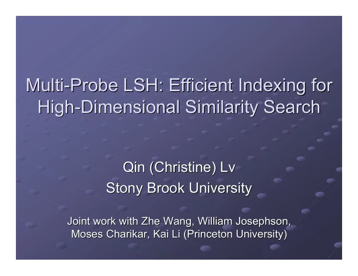
Multi-Probe LSH: Efficient Indexing for Efficient Indexing for Multi-Probe LSH: High-Dimensional Similarity Search High-Dimensional Similarity Search Qin (Christine) (Christine) Lv Lv Qin Stony Brook University Stony Brook University
Multi-Probe LSH: Efficient Indexing for Efficient Indexing for Multi-Probe LSH: High-Dimensional Similarity Search High-Dimensional Similarity Search Qin (Christine) (Christine) Lv Lv Qin Stony Brook University Stony Brook University Joint work with Zhe Zhe Wang, William Wang, William Josephson Josephson, , Joint work with Moses Charikar Charikar, Kai Li (Princeton University) , Kai Li (Princeton University) Moses
Motivations Motivations Massive amounts of feature-rich data Massive amounts of feature-rich data Audio, video, digital photos, sensor data, Audio, video, digital photos, sensor data, … … Fuzzy & high-dimensional Fuzzy & high-dimensional Similarity search Similarity search in high dimensions in high dimensions KNN or ANN in KNN or ANN in feature-vector space feature-vector space Important in various areas Important in various areas Databases, data mining, search engines Databases, data mining, search engines … … 2 2
Ideal Indexing for Similarity Search Ideal Indexing for Similarity Search Accurate Accurate Return Return results that are close to brute-force search results that are close to brute-force search Time efficient Time efficient O(1) or O(log N) query time O(1) or O(log N) query time Space efficient Space efficient Small Small space usage for index space usage for index May fit into main memory even for large datasets May fit into main memory even for large datasets High-dimensional High-dimensional Work well Work well for datasets with high dimensionality for datasets with high dimensionality 3 3
Previous Indexing Methods Previous Indexing Methods K-D tree, R-tree, X-tree, SR-tree … … K-D tree, R-tree, X-tree, SR-tree “ “curse of dimensionality curse of dimensionality” ” Linear scan outperforms when d > 10 Linear scan outperforms when d > 10 [WSB98] [WSB98] Navigating nets [KL04] [KL04] , cover tree , cover tree [BKL06] [BKL06] Navigating nets Based on Based on “ “intrinsic dimensionality intrinsic dimensionality” ” Do not perform well with high intrinsic dimensionality Do not perform well with high intrinsic dimensionality Locality sensitive hashing (LSH) sensitive hashing (LSH) Locality 4 4
Outline Outline Motivations Motivations Locality sensitive hashing (LSH) Locality sensitive hashing (LSH) Basic Basic LSH, LSH, entropy-based LSH entropy-based LSH Multi-probe LSH indexing Multi-probe LSH indexing Step-wise probing, query-directed probing Step-wise probing, query-directed probing Evaluations Evaluations Conclusions & future work Conclusions & future work 5 5
LSH: Locality Sensitive Hashing LSH: Locality Sensitive Hashing cr (r, cr cr, p , p 1 , p 2 )-sensitive [IM98] [IM98] (r, 1 , p 2 )-sensitive q If If D(q,p) < r D(q,p) < r , then , then Pr [h(q) Pr [h(q)=h =h(p)] >= p (p)] >= p 1 r 1 If If D(q,p) > D(q,p) > cr cr , then , then Pr [h(q) Pr [h(q)=h =h(p)] <= p (p)] <= p 2 2 i.e. i.e. closer objects have higher collision probability closer objects have higher collision probability LSH based on based on p p -stable -stable distributions distributions [DIIM04] [DIIM04] LSH w w : slot width : slot width a v b � + � � h b ( v ) = h � � a , w � � w w w Slot 1 Slot 2 Slot 3 6 6
LSH for Similarity Search LSH for Similarity Search False positive False positive h2 Intersection of Intersection of multiple multiple hashes hashes q w False negative False negative w Union of Union of multiple multiple w h1 hashes hashes w w w 7 7
Basic LSH Indexing Basic LSH Indexing q [IM98, GIM99, DIIM04] [IM98, GIM99, DIIM04] M hash functions per table hash functions per table M g i ( v ) = ( h i,1 ( v ) , …, h i,M ( v ) ) L hash tables hash tables L G = { g 1 , …, g L } g L (q) Issues: Issues: g 1 (q) Large number of tables Large number of tables g i (q) L > 100 in L > 100 in [GIM99] [GIM99] L > 500 in L > 500 in [Buhler01] [Buhler01] g 1 g i g L Impractical for large datasets 8 8
Entropy-Based LSH Indexing Entropy-Based LSH Indexing p 4 [Panigrahy Panigrahy, SODA , SODA’ ’06] 06] p 1 [ q R q Randomly perturb q q Randomly perturb p 2 p 3 at distance R R at distance Check hash buckets Check hash buckets of perturbed points of perturbed points g 1 (p 1 ) g L (q) Issues: Issues: g 1 (q) Difficult to choose Difficult to choose R R g i (p 1 ) g L (p 1 ) Duplicate buckets Duplicate buckets g i (q) Inefficient probing g 1 g i g L 9 9
Outline Outline Motivations Motivations Locality Sensitive Hashing (LSH) Locality Sensitive Hashing (LSH) Basic LSH, entropy-based LSH Basic LSH, entropy-based LSH Multi-probe LSH indexing Multi-probe LSH indexing Step-wise probing, query-directed probing Step-wise probing, query-directed probing Evaluations Evaluations Conclusions & future work Conclusions & future work 10 10
Multi-Probe LSH Indexing Multi-Probe LSH Indexing Probes multiple hash buckets per table Probes multiple hash buckets per table Perturbs directly on hash values Perturbs directly on hash values Check left and right slots Check left and right slots Perturbation vector Perturbation vector ∆ g(q) = (2, 5, 3), 5, 3), ∆ = (-1, 1, 0), = (-1, 1, 0), g(q) = (2, q g(q) + ∆ = (1, 6, 3) = (1, 6, 3) g(q) + h w w w Systematic probing Systematic probing 4 h(q) = 5 6 ( ( ∆ 1 , ∆ 2 , ∆ 3 , ∆ 4 , … ) 11 11
Multi-Probe LSH Indexing Multi-Probe LSH Indexing ? probing sequence: A carefully derived A carefully derived ( ∆ 1 , ∆ 2 , ∆ 3 , ∆ 4 , … ) q probing sequence probing sequence Advantages Advantages Fast probing sequence Fast probing sequence generation generation g L (q) g 1 (q)+ ∆ 1 No duplicate buckets No duplicate buckets g 1 (q) g i (q)+ ∆ 2 More effective in finding More effective in finding g L (q)+ ∆ 3 similar objects similar objects g i (q) g i (q)+ ∆ 4 g 1 g i g L 12 12
Step-Wise Probing Step-Wise Probing Given q q ’ ’s s hash values hash values Given g(q)=(3,2,5) ∆ = (0,0,1) 1-step buckets (2,2,5) (4,2,5) (3,2,6) ∆ = (-1,-1,0) 2-step buckets (2,1,5) (2,2,6) (3,3,6) Intuitions Intuitions WRONG! 1-step buckets better than 2-step buckets 1-step buckets better than 2-step buckets All 1-step buckets are equally good All 1-step buckets are equally good 13 13
Success Probability Estimation Success Probability Estimation Hashed position within slot matters! Hashed position within slot matters! Estimation based on x x i (-1) and x i (1) Estimation based on i (-1) and x i (1) 14 14
Query-Directed Probing Query-Directed Probing 0.7 0.3 g(q) = (h 1 (q), h 2 (q), h 3 (q)) = (2, 5, 1) h 1 (q) = 2 0.4 0.6 { 0.2, 0.3, 0.4, 0.6, 0.7, 0.8 } h 2 (q) = 5 0.2 0.8 { x 3 (-1), x 1 (1), x 2 (-1), x 2 (1), x 1 (-1), x 3 (1) } h 3 (q) = 1 { 0.2 } { 0.2, 0.3 } { 0.2, 0.3, 0.4 } { 0.2 } ∆ 1 = (0, 0, -1) (2, 5, 0) { 0.3 } ∆ 2 = (1, 0, 0) (3, 5, 1) { 0.2, 0.4 } { 0.3 } { 0.3, 0.4 } { 0.2, 0.3 } ∆ 3 = (1, 0, -1) (3, 5, 0) { 0.4 } 15 15
Outline Outline Motivations Motivations Locality Sensitive Hashing (LSH) Locality Sensitive Hashing (LSH) Basic LSH, entropy-based LSH Basic LSH, entropy-based LSH Multi-probe LSH indexing Multi-probe LSH indexing Step-wise probing, query-directed probing Step-wise probing, query-directed probing Evaluations Evaluations Conclusions & future work Conclusions & future work 16 16
Evaluations Evaluations Multi-probe vs. basic vs. entropy-based Multi-probe vs. basic vs. entropy-based Tradeoff among space, speed and quality Tradeoff among space, speed and quality Space reduction Space reduction Query-directed vs. step-wise probing Query-directed vs. step-wise probing Tradeoff between search quality and Tradeoff between search quality and number of probes number of probes 17 17
Evaluation Methodology Evaluation Methodology Dataset Dataset #objects #objects #dimensions #dimensions Web images Web images 1.3 million 64 64 1.3 million Switchboard audio Switchboard audio 2.6 million 2.6 million 192 192 Benchmarks Benchmarks 100 random queries, top K results 100 random queries, top K results Evaluation metrics Evaluation metrics I R Search quality: recall, error ratio Search quality: recall, error ratio Search speed: query latency Search speed: query latency Space usage: #hash tables Space usage: #hash tables recall =|I ∩ R| / |I| 18 18
Multi-Probe vs. Basic vs. Entropy Multi-Probe vs. Basic vs. Entropy Multi-probe LSH achieves higher recall with fewer hash tables 19 19
Space Savings of Multi-Probe LSH Space Savings of Multi-Probe LSH 30 11 2 14x - 18x fewer tables than basic LSH 5x - 8x fewer tables than entropy LSH 20 20
Multi-Probe vs. Entropy-Based vs. Entropy-Based Multi-Probe Multi-probe LSH uses much fewer number of probes 21 21
Query-Directed vs. Step-Wise Probing Query-Directed vs. Step-Wise Probing 250 150 20 10 Query-directed probing uses 10x fewer number of probes 22 22
Recommend
More recommend
Explore More Topics
Stay informed with curated content and fresh updates.

