Bayesian Learning l A powerful approach in machine learning l Combine - PowerPoint PPT Presentation

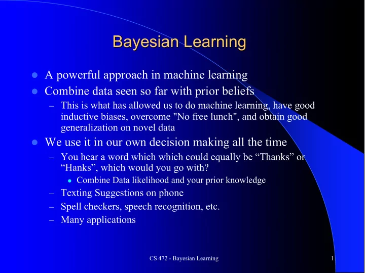
Bayesian Learning l A powerful approach in machine learning l Combine data seen so far with prior beliefs – This is what has allowed us to do machine learning, have good inductive biases, overcome "No free lunch", and obtain good generalization on novel data l We use it in our own decision making all the time – You hear a word which which could equally be “Thanks” or “Hanks”, which would you go with? l Combine Data likelihood and your prior knowledge – Texting Suggestions on phone – Spell checkers, speech recognition, etc. – Many applications CS 472 - Bayesian Learning 1

Bayesian Classification l P ( c | x ) - Posterior probability of output class c given the input vector x l The discriminative learning algorithms we have learned so far try to approximate this directly l P ( c | x ) = P ( x | c ) P ( c )/ P ( x ) Bayes Rule l Seems like more work but often calculating the right hand side probabilities can be relatively easy and advantageous l P ( c ) - Prior probability of class c – How do we know? Just count up and get the probability for the Training Set – Easy! – l P ( x | c ) - Probability “likelihood” of data vector x given that the output class is c We will discuss ways to calculate this likelihood – l P ( x ) - Prior probability of the data vector x This is just a normalizing term to get an actual probability. In practice we drop – it because it is the same for each class c (i.e. independent), and we are just interested in which class c maximizes P ( c | x ). CS 472 - Bayesian Learning 2

Bayesian Classification Example l Assume we have 100 examples in our Training Set with two output classes Good and Bad, and 80 of the examples are of class good. We want to figure out P ( c | x ) ~ P ( x | c ) P ( c ) l Thus our priors are: CS 472 - Bayesian Learning 3

Bayesian Classification Example l Assume we have 100 examples in our Training Set with two output classes Good and Bad, and 80 of the examples are of class good. l Thus our priors are: – P ( Good ) = .8 – P ( Bad ) = .2 l P ( c | x ) = P ( x | c ) P ( c )/ P ( x ) Bayes Rule l Now we are given an input vector x which has the following likelihoods – P ( x | Good ) = .3 – P ( x | Bad ) = .4 l What should our output be? CS 472 - Bayesian Learning 4

Bayesian Classification Example l Assume we have 100 examples in our Training Set with two output classes Good and Bad, and 80 of the examples are of class good. l Thus our priors are: – P ( Good ) = .8 – P ( Bad ) = .2 l P ( c | x ) = P ( x | c ) P ( c )/ P ( x ) Bayes Rule l Now we are given an input vector x which has the following likelihoods – P ( x | Good ) = .3 – P ( x | Bad ) = .4 l What should our output be? l Try all possible output classes and see which one maximizes the posterior using Bayes Rule: P ( c | x ) = P ( x | c ) P ( c )/ P ( x ) – Drop P ( x ) since it is the same for both – P ( Good | x ) = P ( x | Good ) P ( Good ) = .3 · .8 = .24 – P ( Bad | x ) = P ( x | Bad ) P ( Bad ) = .4 · .2 = .08 CS 472 - Bayesian Learning 5

Bayesian Intuition l Bayesian vs. Frequentist l Bayesian allows us to talk about probabilities/beliefs even when there is little data, because we can use the prior – What is the probability of a nuclear plant meltdown? – What is the probability that BYU will win the national championship? l As the amount of data increases, Bayes shifts confidence from the prior to the likelihood l Requires reasonable priors in order to be helpful l We use priors all the time in our decision making – Unknown coin: probability of heads? (over time?) CS 472 - Bayesian Learning 6

Bayesian Learning of ML Models l Assume H is the hypothesis space, h a specific hypothesis from H , and D is all the training data l P ( h | D ) - Posterior probability of h , this is what we usually want to know in a learning algorithm l P ( h ) - Prior probability of the hypothesis independent of D - do we usually know? Could assign equal probabilities – Could assign probability based on inductive bias (e.g. simple hypotheses have – higher probability) – Thus regularization already in the equation l P ( D ) - Prior probability of the data l P ( D | h ) - Probability “likelihood” of data given the hypothesis This is usually just measured by the accuracy of model h on the data – l P ( h | D ) = P ( D | h ) P ( h )/ P ( D ) Bayes Rule l P ( h | D ) increases with P ( D | h ) and P ( h ). In learning when seeking to discover the best h given a particular D , P ( D ) is the same and can be dropped. CS 472 - Bayesian Learning 7

Bayesian Learning l Learning (finding) the best model the Bayesian way l Maximum a posteriori (MAP) hypothesis l h MAP = argmax h ∈ H P ( h | D ) = argmax h ∈ H P ( D | h ) P ( h )/ P ( D ) = argmax h ∈ H P ( D | h ) P ( h ) l Maximum Likelihood (ML) Hypothesis h ML = argmax h ∈ H P ( D | h ) l MAP = ML if all priors P ( h ) are equally likely (uniform priors) l Note that the prior can be like an inductive bias (i.e. simpler hypotheses are more probable) l For Machine Learning P ( D | h ) is usually measured using the accuracy of the hypothesis on the training data – If the hypothesis is very accurate on the data, that implies that the data is more likely given that particular hypothesis – For Bayesian learning, don't have to worry as much about h overfitting in P ( D | h ) (early stopping, etc.) – Why? CS 472 - Bayesian Learning 8

Bayesian Learning (cont) l Brute force approach is to test each h ∈ H to see which maximizes P ( h | D ) l Note that the argmax is not the real probability since P ( D ) is unknown, but not needed if we're just trying to find the best hypothesis l Can still get the real probability (if desired) by normalization if there is a limited number of hypotheses – Assume only two possible hypotheses h 1 and h 2 – The true posterior probability of h 1 would be 𝑄(𝐸|ℎ 1 )𝑄(ℎ 1 ) 𝑄(ℎ 1 |𝐸) = 𝑄(𝐸|ℎ 1 ) + 𝑄(𝐸|ℎ 2 ) CS 472 - Bayesian Learning 9

Example of MAP Hypothesis l Assume only 3 possible hypotheses in hypothesis space H l Given a data set D which h do we choose? l Maximum Likelihood (ML): argmax h Î H P ( D | h ) l Maximum a posteriori (MAP): argmax h Î H P ( D | h ) P ( h ) H Likelihood Priori Relative Posterior P ( D | h ) P ( h ) P ( D | h ) P ( h ) h 1 .6 .3 .18 h 2 .9 .2 .18 h 3 .7 .5 .35 CS 472 - Bayesian Learning 10

Example of MAP Hypothesis – True Posteriors l Assume only 3 possible hypotheses in hypothesis space H l Given a data set D H Likelihood Priori Relative Posterior True Posterior P ( D | h ) P ( h ) P ( D | h ) P ( h ) P ( D | h ) P ( h )/ P ( D ) h 1 .6 .3 .18 .18/(.18+.18+.35) = .18/.71 = .25 h 2 .9 .2 .18 .18/.71 = .25 h 3 .7 .5 .35 .35/.71 = .50 CS 472 - Bayesian Learning 11

Prior Handles Overfit l Prior can make it so that less likely hypotheses (those likely to overfit) are less likely to be chosen l Similar to the regularizer l Minimize F ( h ) = Error ( h ) + λ·Complexity ( h ) l P ( h | D ) = P ( D | h ) P ( h ) l The challenge is – Deciding on priors – subjective – Maximizing across H which is usually infinite – approximate by searching over "best h 's" in more efficient time CS 472 - Bayesian Learning 12

Minimum Description Length l Information theory shows that the number of bits required to encode a message i is -log 2 p i l Call the minimum number of bits to encode message i with respect to code C : L C ( i ) h MAP = argmax h Î H P ( h ) P ( D | h ) = argmin h Î H - log 2 P ( h ) - log 2 ( D | h ) = argmin h Î H L C 1 ( h ) + L C 2 ( D | h ) l L C 1 ( h ) is a representation of hypothesis l L C 2 ( D | h ) is a representation of the data. Since you already have h all you need is the data instances which differ from h , which are the lists of misclassifications l The h which minimizes the MDL equation will have a balance of a small representation (simple hypothesis) and a small number of errors CS 472 - Bayesian Learning 13

Bayes Optimal Classifier l Best question is what is the most probable classification c for a given instance, rather than what is the most probable hypothesis for a data set l Let all possible hypotheses vote for the instance in question weighted by their posterior (an ensemble approach) - better than the single best MAP hypothesis 𝑄 𝑑 𝑘 ℎ 𝑗 𝑄(𝐸|ℎ 𝑗 )𝑄(ℎ 𝑗 ) 𝑄 𝑑 𝑘 𝐸, 𝐼 = ' 𝑄 𝑑 𝑘 ℎ 𝑗 𝑄(ℎ $ |𝐸) = ' 𝑄(𝐸) ! ! ∈# ! ! ∈# l Bayes Optimal Classification: 𝑑 𝐶𝑏𝑧𝑓𝑡𝑃𝑞𝑢𝑗𝑛𝑏𝑚 = argmax ( 𝑄 𝑑 𝑘 ℎ 𝑗 𝑄(ℎ & |𝐸) = argmax ( 𝑄 𝑑 𝑘 ℎ 𝑗 𝑄(𝐸|ℎ & )𝑄(ℎ & ) ! ! ∈# ! ! ∈# $ " ∈% $ " ∈% l Also known as the posterior predictive CS 472 - Bayesian Learning 14

Example of Bayes Optimal Classification 𝑑 𝐶𝑏𝑧𝑓𝑡𝑃𝑞𝑢𝑗𝑛𝑏𝑚 = argmax ( 𝑄 𝑑 𝑘 ℎ 𝑗 𝑄(ℎ & |𝐸) = argmax ( 𝑄 𝑑 𝑘 ℎ 𝑗 𝑄(𝐸|ℎ & )𝑄(ℎ & ) ! ! ∈# ! ! ∈# $ " ∈% $ " ∈% Assume same 3 hypotheses with priors and posteriors as shown for a data set D l with 2 possible output classes (A and B) Assume novel input instance x where h 1 and h 2 output B and h 3 outputs A for x – l 1/0 output case. Which class wins and what are the probabilities? H Likelihood Prior Posterior P (A) P (B) P ( D | h ) P ( h ) P ( D | h ) P ( h ) h 1 .6 .3 .18 0·.18 = 0 1·.18 = .18 h 2 .9 .2 .18 h 3 .7 .5 .35 Sum CS 472 - Bayesian Learning 15