Multi-Armed Bandit: Learning in Dynamic Systems with Unknown Models - PowerPoint PPT Presentation
1 Multi-Armed Bandit: Learning in Dynamic Systems with Unknown Models Qing Zhao Department of Electrical and Computer Engineering University of California, Davis, CA 95616 Supported by NSF, ARO. c Qing Zhao. Talk at UMD, October, 2011. 2
1 Multi-Armed Bandit: Learning in Dynamic Systems with Unknown Models Qing Zhao Department of Electrical and Computer Engineering University of California, Davis, CA 95616 Supported by NSF, ARO.
c � Qing Zhao. Talk at UMD, October, 2011. 2 Multi-Armed Bandit Multi-Armed Bandit: ◮ N arms and a single player. ◮ Select one arm to play at each time. ◮ i.i.d. reward with Unknown mean θ i . ◮ Maximize the long-run reward. Exploitation v.s. Exploration ◮ Exploitation: play the arm with the largest sample mean. ◮ Exploration: play an arm to learn its reward statistics.
c � Qing Zhao. Talk at UMD, October, 2011. 3 Clinical Trial (Thompson’33) Two treatments with unknown effectiveness:
c � Qing Zhao. Talk at UMD, October, 2011. 4 Dynamic Spectrum Access Dynamic Spectrum Access under Unknown Model: Opportunities ��������� ��������� ��������� ��������� �������� �������� ��������� ��������� ��������� ��������� ��������� ��������� �������� �������� ��������� ��������� ��������� ��������� ��������� ��������� �������� �������� ��������� ��������� Channel 1 ��������� ��������� ��������� ��������� �������� �������� ��������� ��������� t �������� �������� ��������� ��������� ��������� ��������� �������� �������� ��������� ��������� ��������� ��������� �������� �������� ��������� ��������� ��������� ��������� Channel N �������� �������� ��������� ��������� ��������� ��������� t 0 1 2 3 T ◮ N independent channels. ◮ Choose K channels to sense/access in each slot. ◮ Accessing an idle channel results in a unit reward. ◮ Channel occupancy: i.i.d. Bernoulli with unknown mean θ i .
c � Qing Zhao. Talk at UMD, October, 2011. 5 Other Applications of MAB Web Search Internet Advertising/Investment Queueing and Scheduling Multi-Agent Systems λ 2 λ 1
c � Qing Zhao. Talk at UMD, October, 2011. 6 Non-Bayesian Formulation Performance Measure: Regret ∆ = ( θ 1 , · · · , θ N ) : unknown reward means. ◮ Θ ◮ θ (1) T : max total reward (by time T ) if Θ is known. ◮ V π T (Θ) : total reward of policy π by time T . ◮ Regret (cost of learning): N � ( θ (1) − θ ( i ) ) E [ time spent on θ ( i ) ] . ∆ R π = θ (1) T − V π T (Θ) T (Θ) = i =2 Objective : minimize the growth rate of R π T (Θ) with T . sublinear regret = ⇒ maximum average reward θ (1)
c � Qing Zhao. Talk at UMD, October, 2011. 7 Classic Results ◮ Lai&Robbins’85 : θ (1) − θ ( i ) � R ∗ log T as T → ∞ . T (Θ) ∼ I ( θ ( i ) , θ (1) ) i> 1 � �� � KL distance ✷ Optimal policies explicitly constructed for Gaussian, Bernoulli, Poisson, and Laplacian distributions. ◮ Agrawal’95 : ✷ Order-optimal index policies explicitly constructed for Gaussian, Bernoulli, Poisson, Laplacian, and Exponential distributions. ◮ Auer&Cesa-Bianchi&Fischer’02 : ✷ Order-optimal index policies for distributions with finite support.
c � Qing Zhao. Talk at UMD, October, 2011. 8 Classic Policies Key Statistics: ◮ Sample mean ¯ θ i ( t ) ( exploitation ); ◮ Number of plays τ i ( t ) ( exploration ); In the classic policies: ◮ ¯ θ i ( t ) and τ i ( t ) are combined together for arm selection at each t : � 2 log t index = ¯ UCB Policy( Auer et al. :02 ): θ i + τ i ( t ) ◮ A fixed form difficult to adapt to different reward models.
c � Qing Zhao. Talk at UMD, October, 2011. 9 Limitations ◮ Limitations of the Classic Policies : ✷ Reward distributions limited to finite support or specific cases; ✷ A single player (equivalently, centralized multiple players); ✷ i.i.d. or rested Markov reward over successive plays of each arm.
c � Qing Zhao. Talk at UMD, October, 2011. 10 Recent Results ◮ Limitations of the Classic Policies : ✷ Reward distributions limited to finite support or specific cases; ✷ A single player (equivalently, centralized multiple players); ✷ i.i.d. or rested Markov reward over successive plays of each arm. ◮ Recent results: policies with a tunable parameter capable of handling ✷ a more general class of reward distributions (including heavy-tailed); ✷ decentralized MAB with partial reward observations; ✷ restless Markovian reward model.
c � Qing Zhao. Talk at UMD, October, 2011. 11 General Reward Distributions
c � Qing Zhao. Talk at UMD, October, 2011. 12 DSEE Deterministic Sequencing of Exploration and Exploitation (DSEE): ◮ Time is partitioned into interleaving exploration and exploitation sequences. t = 1 T ✷ Exploration: play all arms in round-robin. ✷ Exploitation: play the arm with the largest sample mean. ◮ A tunable parameter: the cardinality of the exploration sequence ✷ can be adjusted according to the “hardness” of the reward distributions.
c � Qing Zhao. Talk at UMD, October, 2011. 13 The Optimal Cardinality of Exploration The Cardinality of Exploration: ✷ a lower bound of the regret order; ✷ should be the min x so that regret in exploitation is no larger than x . ◮ O (log T ) ? 0 0 50 100 150 200 250 300 350 400 450 500 Time (T) √ T ) ? ◮ O ( 0 0 50 100 150 200 250 300 350 400 450 500 Time (T)
c � Qing Zhao. Talk at UMD, October, 2011. 14 Performance of DSEE When moment generating functions of { f i ( x ) } are properly bounded around 0 : 3.5 ◮ ∃ ζ > 0 , u 0 > 0 s.t. ∀ u with | u | ≤ u 0 , 3 E [exp(( X − θ ) u )] ≤ exp( ζu 2 / 2) Chi−square Moment−Generating Function G(u) Gaussian (large variance) Gaussian (small variance) 2.5 Uniform ◮ DSEE achieves the optimal regret 2 order O (log T ) . 1.5 1 ◮ Achieve a regret arbitrary close to log- arithmic w.o. any knowledge. 0.5 −0.4 −0.3 −0.2 −0.1 0 0.1 0.2 0.3 0.4 u When { f i ( x ) } are heavy-tailed distributions: ◮ The moments of { f i ( x ) } exist only up to the p th order; ◮ DSEE achieves regret order O ( T 1 /p ) .
c � Qing Zhao. Talk at UMD, October, 2011. 15 Basic Idea in Regret Analysis Convergence Rate of the Sample Mean: ◮ Chernoff-Hoeffding Bound (’63): for distributions w. finite support [ a, b ] , Pr( | X s − θ | ≥ δ ) ≤ 2 exp( − 2 δ 2 s/ ( b − a ) 2 ) . ◮ Chernoff-Hoeffding-Agrawal Bound (’95): for distributions w. bounded MGF around 0 , Pr( | X s − θ | ≥ δ ) ≤ 2 exp( − cδ 2 s ) , ∀ δ ∈ [0 , ζu 0 ] , c ∈ (0 , 1 / (2 ζ )] . ◮ Chow’s Bound (’75): for distributions having the p th ( p > 1) moment, Pr( | X s − θ | > ǫ ) = o ( s 1 − p ) .
c � Qing Zhao. Talk at UMD, October, 2011. 16 Decentralized Bandit with Multiple Players
c � Qing Zhao. Talk at UMD, October, 2011. 17 Distributed Spectrum Sharing Opportunities ��������� ��������� ��������� ��������� �������� �������� ��������� ��������� ��������� ��������� ��������� ��������� �������� �������� ��������� ��������� ��������� ��������� ��������� ��������� �������� �������� ��������� ��������� Channel 1 ��������� ��������� ��������� ��������� �������� �������� ��������� ��������� t �������� �������� ��������� ��������� ��������� ��������� �������� �������� ��������� ��������� ��������� ��������� �������� �������� ��������� ��������� ��������� ��������� Channel N �������� �������� ��������� ��������� ��������� ��������� t 0 1 2 3 T ◮ N channels, M ( M < N ) distributed secondary users (no info exchange). ◮ Primary occupancy of channel i : i.i.d. Bernoulli with unknown mean θ i : ◮ Users accessing the same channel collide; no one receives reward. ◮ Objective: decentralized policy for optimal network-level performance.
Recommend
More recommend
Explore More Topics
Stay informed with curated content and fresh updates.
