Multi-Armed Bandits: Non-adaptive and Adaptive Sampling Instructor: - PDF document

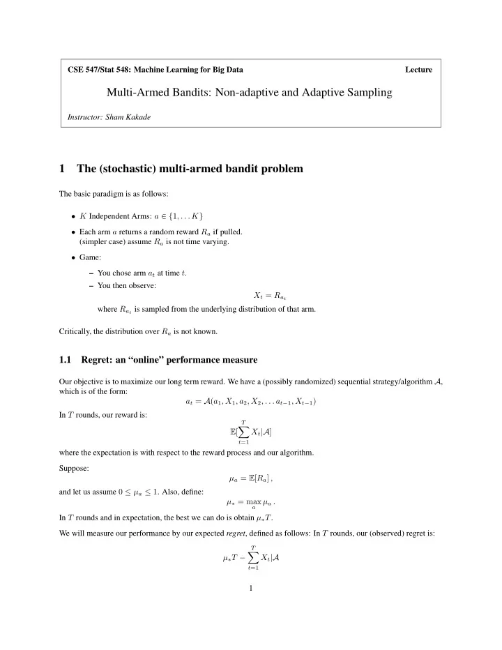
CSE 547/Stat 548: Machine Learning for Big Data Lecture Multi-Armed Bandits: Non-adaptive and Adaptive Sampling Instructor: Sham Kakade 1 The (stochastic) multi-armed bandit problem The basic paradigm is as follows: • K Independent Arms: a ∈ { 1 , . . . K } • Each arm a returns a random reward R a if pulled. (simpler case) assume R a is not time varying. • Game: – You chose arm a t at time t . – You then observe: X t = R a t where R a t is sampled from the underlying distribution of that arm. Critically, the distribution over R a is not known. 1.1 Regret: an “online” performance measure Our objective is to maximize our long term reward. We have a (possibly randomized) sequential strategy/algorithm A , which is of the form: a t = A ( a 1 , X 1 , a 2 , X 2 , . . . a t − 1 , X t − 1 ) In T rounds, our reward is: T � E [ X t |A ] t =1 where the expectation is with respect to the reward process and our algorithm. Suppose: µ a = E [ R a ] , and let us assume 0 ≤ µ a ≤ 1 . Also, define: µ ∗ = max µ a . a In T rounds and in expectation, the best we can do is obtain µ ∗ T . We will measure our performance by our expected regret , defined as follows: In T rounds, our (observed) regret is: T � µ ∗ T − X t |A t =1 1

and our expected regret is: � T � � µ ∗ T − E X t |A t =1 where the expectation is with the randomness in our outcomes (and possibly our algorithm if it is randomized). 1.2 Caveat: Our presentation in these notes will be loose in terms of log( · ) factors, in both K and T . There are multiple good treatments that provide improvements in terms of these factors. 2 Review: Hoeffding’s bound With N samples, denote the sample mean as: µ = 1 � ˆ X t . N t Lemma 2.1. Supposing that the X t ’s have an i.i.d. distribution and are bounded between 0 and 1 , then, with proba- bility greater than 1 − δ , we have that � log(2 /δ ) | ˆ µ − µ | ≤ . 2 N 3 Warmup: A non-adaptive strategy Suppose we first pull each arm τ times, in an exploration phase. Then, for the remainder of the T steps, we pull the arm which had the best observed reward during the exploration phase. By the union bound, with probability greater than 1 − δ , for all actions a , � log( K/δ ) | ˆ µ a − µ a | ≤ O . τ To see this, we simply make our error probability to be δ/K , to the total error probability is δ . Thus all the confidence intervals will hold. During the exploration rounds, our cumulative regret is at most Kτ , a trivial upper bound. During the exploitation rounds, let us bound our cumulative regret for the remainder of T − Kτ . Note that for the arm i that we pull, we must have that: µ i ≥ ˆ ˆ µ i ∗ where i ∗ is an optimal arm. This implies that � log( K/δ ) µ i ≥ µ ∗ − c τ where c is a universal constant. To see this, note that by construction of the algorithm ˆ µ i ≥ ˆ µ i ∗ , which implies µ i ≥ ˆ µ i − | ˆ µ i − µ i | ≥ ˆ µ i ∗ − | ˆ µ i − µ i | ≥ µ i ∗ − | ˆ µ i − µ i | − | ˆ µ i ∗ − µ i ∗ | , and the claim follows using the confidence interval bounds. 2

Hence, our total regret is: T � log( K/δ ) � µ ∗ T − X t ≤ τK + O ( T − Kτ ) τ t =1 Now let us optimize for τ . Lemma 3.1. (Regret of the non-adaptive strategy) The total expected regret of the non-adaptive strategy is: � T � � ≤ cK 1 / 3 T 2 / 3 (log T ) 1 / 3 µ ∗ T − E X t t =1 where c is a universal constant. Proof. Choose τ = K 2 / 3 T 2 / 3 and δ = 1 /T 2 . Note that with probability greater than 1 − 1 /T 2 , our regret is bounded by ( K 1 / 3 T 2 / 3 (log( KT )) 1 / 3 ) . Also, if we ’fail’, the largest regret we can pay is T , and this occurs with probability less than 1 /T 2 , so the reget is: Pr( no failure event ) ∗ K 1 / 3 T 2 / 3 (log( KT )) 1 / 3 + Pr( failure event ) T ≤ exp. regret c (1 − 1 /T 2 ) K 1 / 3 T 2 / 3 (log( KT )) 1 / 3 + 1 ≤ T . This shows that the regret is bounded as O ( K 1 / 3 T 2 / 3 (log( KT )) 1 / 3 ) . For T > K , log( KT ) ≤ 2 log T (and for K < T , the claimed regret bound is trivially true). This completes the proof (for a different universal constant). 3.1 A (minimax) optimal adaptive algorithm We will now provide an optimal (up to log factors) algorithms (optimal under the i.i.d. assumption for the rewards are distributed and using that the rewards are upper bounded by 1 ). Let N a,t be the number of times we pulled arm a up to time t . The question is what arm should pull a time t + 1 ? 3.2 Confidence bounds If we don’t care about log factors, then the following is a straightforward argument to see that our confidence bounds will simultaneously hold for all times t (from 0 to ∞ ) and all K arms. Lemma 3.2. With probability greater than 1 − δ , we will have that for all times t ≥ K , all a ∈ [ K ] , � log( t/δ ) | ˆ µ a,t − µ a | ≤ c N a,t where c is a universal constant. Proof. We will actually prove a stronger statement: suppose that we observe the outcome of every arm, we will first provide a probabilistic statement for the confidence intervals of all the arms (and for all sample sizes). Let us apply Hoeffding’s bound with an error probability of δ/ ( Kτ 2 ) . Specifically, for the arm a with τ samples, we have that with probability greater than 1 − δ/ ( Kτ 2 ) : � log( τK/δ ) | ˆ µ a,τ − µ a | ≤ c τ 3

(by a straightforward application of Hoeffding’s bound). Now that the total error probability over all arms an over sample size τ is: ∞ δ � � Kτ 2 = δπ 2 / 6 a τ =0 (the π 2 / 6 is from Basel’s problem). Note the sum is finite, which means the error total probability for all of these confidence intervals is less than a constant ∗ δ . We have thus shown the following (note the quantifiers): with probability greater than 1 − δ , that for all arms a and all sample sizes τ ≥ 1 that: � log( τK/δ ) | ˆ µ a,τ − µ a | ≤ c , τ (for a possibility different constant c ). Observe that the confidence bounds that any algorithm uses at time t is due to having N a,t samples, so we can now apply the above bound in this case, where: � � log( N a,t K/δ ) log( tK/δ ) c ≤ c N a,t N a,t since N a,t ≤ t . This shows that these confidence bounds are valid for all times t and all arms a . The proof is completed by nothing for t ≥ K , log( Kt ) ≤ 2 log t . 3.3 The Upper Confidence Bound (UCB) Algorithm • At each time t , – Pull arm: � log( t/δ ) a t = arg max ˆ µ a,t + c N a,t := arg max ˆ µ a,t + ConfBound a,t (where c ≤ 10 is a constant). – Observe reward X t . – Update µ a,t , N a,t , and ConfBound a,t . With probability greater than 1 − δ all the confidence bounds will hold for all arms and all times t . 3.4 Analysis of UCB If pull arm a at time t , what is our instantaneous regret, i.e. what is: µ ∗ − µ a t ≤ ? Let i ∗ be an optimal arm. Note by construction of the algorithm we have, if we pull arm a at time t , then: ˆ ˆ µ a,t + ConfBound a,t ≥ ˆ µ i ∗ + ConfBound i ∗ ≥ µ i ∗ , the last step follows due to that µ i ∗ is contained within the confidence interval for i ∗ . Using this we have that: µ a t ≥ µ a,t − ConfBound a,t ˆ ≥ µ i ∗ − 2 ConfBound a,t ˆ 4

Theorem 3.3. (UCB regret) The total expected regret of UCB is: � T � � � µ ∗ T − E X t ≤ c KT log T t =1 for an appropriately chosen universal constant c . Proof. The expected regret is bounded as: � T � � � µ ∗ T − E X t ≤ 2 ConfBound a,t t =1 t � log( t/δ ) � ≤ 2 c N a,t t � ≤ 2 c log( T/δ ) N a,T . (1) Note the following constraint on the N a,T ’s must hold: � N a,T = T a One can now show the worst case setting of N a,T that makes Equation 1 as large as possible (subject to this constraint on the N a,T ’s) is when N a,t = T/K . Finally, to obtain the expected regret bound, the proof is identical to that of the previous argument (in the non-adaptive case, where we choose δ = 1 /T 2 ). 5