Motivation For continuous spaces: often no analytical formulas for - PDF document

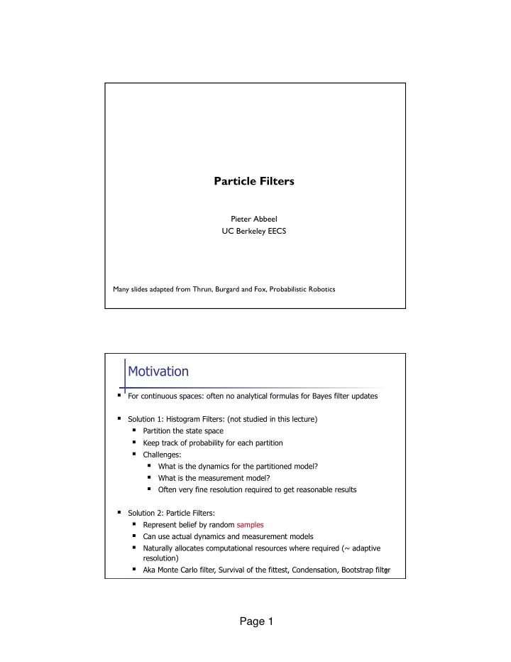
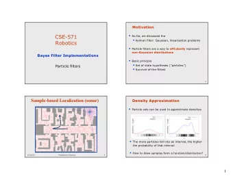
Particle Filters Pieter Abbeel UC Berkeley EECS Many slides adapted from Thrun, Burgard and Fox, Probabilistic Robotics Motivation § For continuous spaces: often no analytical formulas for Bayes filter updates § Solution 1: Histogram Filters: (not studied in this lecture) § Partition the state space § Keep track of probability for each partition § Challenges: § What is the dynamics for the partitioned model? § What is the measurement model? § Often very fine resolution required to get reasonable results § Solution 2: Particle Filters: § Represent belief by random samples § Can use actual dynamics and measurement models § Naturally allocates computational resources where required (~ adaptive resolution) § Aka Monte Carlo filter, Survival of the fittest, Condensation, Bootstrap filter 2 Page 1 �

Sample-based Localization (sonar) Problem to be Solved n Given a sample-based representation 1 , x t 2 ,..., x t N } S t = { x t of Bel (x t ) = P(x t | z 1 , …, z t , u 1 , …, u t ) 1 , x t + 1 2 ,..., x t + 1 N } Find a sample-based representation S t + 1 = { x t + 1 of Bel (x t+1 ) = P(x t+1 | z 1 , …, z t , z t+1 , u 1 , …, u t+1 ) Page 2 �

Dynamics Update n Given a sample-based representation 1 , x t 2 ,..., x t N } S t = { x t of Bel (x t ) = P(x t | z 1 , …, z t , u 1 , …, u t ) Find a sample-based representation of P(x t+1 | z 1 , …, z t , u 1 , …, u t+1 ) n Solution: n For i=1, 2, …, N n Sample x i t+1 from P(X t+1 | X t = x i t ) Sampling Intermezzo Page 3 �

Observation update 1 , x t + 1 2 ,..., x t + 1 N } n Given a sample-based representation of { x t + 1 P(x t+1 | z 1 , …, z t ) Find a sample-based representation of P(x t+1 | z 1 , …, z t , z t+1 ) = C * P(x t+1 | z 1 , …, z t ) * P(z t+1 | x t+1 ) n Solution: n For i=1, 2, …, N n w (i) t+1 = w (i) t * P(z t+1 | X t+1 = x (i) t+1 ) the distribution is represented by the weighted set of samples n 1 , w t + 1 1 > , < x t + 1 2 , w t + 1 2 > ,..., < x t + 1 N , w t + 1 N > } { < x t + 1 Sequential Importance Sampling (SIS) Particle Filter Sample x 1 1 , x 2 1 , …, x N 1 from P(X 1 ) n Set w i 1 = 1 for all i=1,…,N n For t=1, 2, … n Dynamics update: n n For i=1, 2, …, N n Sample x i t+1 from P(X t+1 | X t = x i t ) Observation update: n n For i=1, 2, …, N n w i t+1 = w i t * P(z t+1 | X t+1 = x i t+1 ) At any time t, the distribution is represented by the weighted set of samples n { < x i t , w i t > ; i=1,…,N} Page 4 �

SIS particle filter major issue n The resulting samples are only weighted by the evidence n The samples themselves are never affected by the evidence à Fails to concentrate particles/computation in the high probability areas of the distribution P(x t | z 1 , …, z t ) Sequential Importance Resampling (SIR) n At any time t, the distribution is represented by the weighted set of samples { < x i t , w i t > ; i=1,…,N} à Sample N times from the set of particles à The probability of drawing each particle is given by its importance weight à More particles/computation focused on the parts of the state space with high probability mass Page 5 �

1. Algorithm particle_filter ( S t-1 , u t , z t ): 2. S , 0 = ∅ η = t 3. For Generate new samples i 1 … n = 4. Sample index j(i) from the discrete distribution given by w t-1 5. Sample from using and i j ( i ) x p ( x t | x t ! 1 , u t ) x − u t t t 1 6. i i Compute importance weight w = p ( z | x ) t t t i 7. w Update normalization factor η = η + t 8. i i Insert S S { x , w } = ∪ < > t t t t 9. For i 1 … n = i i 10. w = w / Normalize weights η t t Particle Filters Page 6 �

Sensor Information: Importance Sampling Bel ( x ) p ( z | x ) Bel − ( x ) ← α p ( z | x ) Bel − ( x ) α w p ( z | x ) ← = α Bel ( x ) − Robot Motion Bel ( x ) p ( x | u x ' ) Bel ( x ' ) d x ' − ← ∫ , Page 7 �

Sensor Information: Importance Sampling Bel ( x ) p ( z | x ) Bel − ( x ) ← α p ( z | x ) Bel − ( x ) α w p ( z | x ) ← = α Bel ( x ) − Robot Motion Bel ( x ) p ( x | u x ' ) Bel ( x ' ) d x ' − ← ∫ , Page 8 �

20 21 Page 9 �

22 23 Page 10 �

24 25 Page 11 �

26 27 Page 12 �

28 29 Page 13 �

30 31 Page 14 �

32 33 Page 15 �

34 35 Page 16 �

36 37 Page 17 �

Summary – Particle Filters Particle filters are an implementation of recursive § Bayesian filtering They represent the posterior by a set of weighted § samples They can model non-Gaussian distributions § Proposal to draw new samples § Weight to account for the differences between the § proposal and the target 42 Summary – PF Localization In the context of localization, the particles are propagated § according to the motion model. They are then weighted according to the likelihood of the § observations. In a re-sampling step, new particles are drawn with a § probability proportional to the likelihood of the observation. 43 Page 18 �