Motion Planning n Problem n Given start state x S , goal state x G n - PDF document
Motion Planning Pieter Abbeel UC Berkeley EECS Many images from Lavalle, Planning Algorithms Motion Planning n Problem n Given start state x S , goal state x G n Asked for: a sequence of control inputs that leads from start to goal
Motion Planning Pieter Abbeel UC Berkeley EECS Many images from Lavalle, Planning Algorithms Motion Planning n Problem n Given start state x S , goal state x G n Asked for: a sequence of control inputs that leads from start to goal n Why tricky? n Need to avoid obstacles n For systems with underactuated dynamics: can’t simply move along any coordinate at will n E.g., car, helicopter, airplane, but also robot manipulator hitting joint limits Page 1 �
Solve by Nonlinear Optimization for Control? Could try by, for example, following formulation: n X t can encode obstacles Or, with constraints, (which would require using an infeasible method): n Can work surprisingly well, but for more complicated problems with longer n horizons, often get stuck in local maxima that don’t reach the goal Examples n Helicopter path planning n Swinging up cart-pole n Acrobot Page 2 �
Examples Examples Page 3 �
Examples Motion Planning: Outline n Configuration Space n Probabilistic Roadmap n Boundary Value Problem n Sampling n Collision checking n Rapidly-exploring Random Trees (RRTs) n Smoothing Page 4 �
Configuration Space (C-Space) = { x | x is a pose of the robot} n obstacles à configuration space obstacles Workspace Configuration Space (2 DOF: translation only, no rotation) free space obstacles Motion planning Page 5 �
Probabilistic Roadmap (PRM) Free/feasible space Space ℜ n forbidden space 11 Probabilistic Roadmap (PRM) Configurations are sampled by picking coordinates at random 12 Page 6 �
Probabilistic Roadmap (PRM) Configurations are sampled by picking coordinates at random 13 Probabilistic Roadmap (PRM) Sampled configurations are tested for collision 14 Page 7 �
Probabilistic Roadmap (PRM) The collision-free configurations are retained as milestones 15 Probabilistic Roadmap (PRM) Each milestone is linked by straight paths to its nearest neighbors 16 Page 8 �
Probabilistic Roadmap (PRM) Each milestone is linked by straight paths to its nearest neighbors 17 Probabilistic Roadmap (PRM) The collision-free links are retained as local paths to form the PRM 18 Page 9 �
Probabilistic Roadmap (PRM) The start and goal configurations are included as milestones g s 19 Probabilistic Roadmap (PRM) The PRM is searched for a path from s to g g s 20 Page 10 �
Probabilistic Roadmap n Initialize set of points with x S and x G n Randomly sample points in configuration space n Connect nearby points if they can be reached from each other n Find path from x S to x G in the graph n alternatively: keep track of connected components incrementally, and declare success when x S and x G are in same connected component PRM example Page 11 �
PRM example 2 PRM: Challenges 1. Connecting neighboring points: Only easy for holonomic systems (i.e., for which you can move each degree of freedom at will at any time). Generally requires solving a Boundary Value Problem Typically solved without collision checking; later verified if valid by collision checking 2. Collision checking: Often takes majority of time in applications (see Lavalle) 3. Sampling: how to sample uniformly (or biased according to prior information) over configuration space? Page 12 �
Sampling n How to sample uniformly at random from [0,1] n ? n Sample uniformly at random from [0,1] for each coordinate n How to sample uniformly at random from the surface of the n-D unit sphere? n Sample from n-D Gaussian à isotropic; then just normalize n How to sample uniformly at random for orientations in 3-D? PRM’s Pros and Cons n Pro: n Probabilistically complete: i.e., with probability one, if run long the graph will contain a solution path if one exists. n Cons: n Required to solve 2 point boundary value problem n Build graph over state space but no particular focus on generating a path Page 13 �
Rapidly exploring Random Trees n Basic idea: n Build up a tree through generating “next states” in the tree by executing random controls n However: not exactly above to ensure good coverage Rapidly-exploring Random Trees (RRT) RANDOM_STATE(): often uniformly at random over space with probability 99%, and the goal state with probability 1%, this ensures it attempts to connect to goal semi-regularly Page 14 �
RRT Practicalities n NEAREST_NEIGHBOR( x rand , T): need to find (approximate) nearest neighbor efficiently n KD Trees data structure (upto 20-D) [e.g., FLANN] n Locality Sensitive Hashing n SELECT_INPUT ( x rand , x near ) n Two point boundary value problem n If too hard to solve, often just select best out of a set of control sequences. This set could be random, or some well chosen set of primitives. RRT Extension No obstacles, holonomic: n With obstacles, holonomic: n Non-holonomic: approximately (sometimes as approximate as picking n best of a few random control sequences) solve two-point boundary value problem Page 15 �
Growing RRT Bi-directional RRT Volume swept out by unidirectional RRT: n x S x G Volume swept out by bi-directional RRT: n x S x G Difference becomes even more pronounced in higher dimensions n Page 16 �
Multi-directional RRT n Planning around obstacles or through narrow passages can often be easier in one direction than the other Resolution-Complete RRT (RC-RRT) n Issue: nearest points chosen for expansion are (too) often the ones stuck behind an obstacle RC-RRT solution: Choose a maximum number of times, m, you are willing to try to expand each node n For each node in the tree, keep track of its Constraint Violation Frequency (CVF) n Initialize CVF to zero when node is added to tree n Whenever an expansion from the node is unsuccessful (e.g., per hitting an obstacle): n n Increase CVF of that node by 1 n Increase CVF of its parent node by 1/m, its grandparent 1/ m 2 , … When a node is selected for expansion, skip over it with probability CVF/m n Page 17 �
Smoothing Randomized motion planners tend to find not so great paths for execution: very jagged, often much longer than necessary. à In practice: do smoothing before using the path n Shortcutting: n along the found path, pick two vertices x t1 , x t2 and try to connect them directly (skipping over all intermediate vertices) n Nonlinear optimization for optimal control n Allows to specify an objective function that includes smoothness in state, control, small control inputs, etc. Example: Swing up Pendulum Page 18 �
Example: Swing up Acrobot Page 19 �
Recommend
More recommend
Explore More Topics
Stay informed with curated content and fresh updates.
