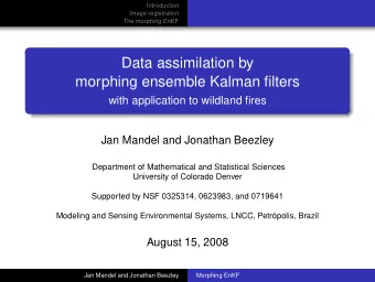
Morphing ensemble Kalman filter and applications Jan Mandel and - PowerPoint PPT Presentation

Data assimilation Applications Software Morphing ensemble Kalman filter and applications Jan Mandel and Jonathan D. Beezley Center for Computational Mathematics Department of Mathematical and Statistical Sciences University of Colorado Denver Supported by NSF grants CNS-0623983 and ATM-0719641 Institute of Computer Science Czech Academy of Sciences Prague, June 3, 2009 Jan Mandel and Jonathan D. Beezley Morphing EnKF

Data assimilation Applications Software Outline Data assimilation 1 EnKF Registration and morphing Applications 2 Wildfire Epidemic spread Other applications Software 3 Software structure Available software Future developments Jan Mandel and Jonathan D. Beezley Morphing EnKF

Data assimilation EnKF Applications Registration and morphing Software Data assimilation Model must support the assimilation cycle: export, modify, and import state the state must be described: what, when, where changes to the state must be meaningful: no discrete datastructures (such as tracers) Data must have error estimate must have metadata: what, when, where Observation function connects the data and the model creates synthetic data from model state to compare Data assimilation algorithm adjusts the state to match the data balances the uncertainty in the data and in the state Jan Mandel and Jonathan D. Beezley Morphing EnKF

Data assimilation EnKF Applications Registration and morphing Software The Ensemble Kalman Filter (EnKF) uses an ensemble of simulations to estimate model uncertainty by sample covariance converges to Kalman Filter (optimal filter) in large ensemble limit and the Gaussian case uses the model as a black box adjusts the state by making linear combinations of ensemble members (OK, locally in local versions of the filter, but still only linear combinations) if it cannot match the data by making the linear combinations, it cannot track the data probability distributions close to normal needed for proper operation Jan Mandel and Jonathan D. Beezley Morphing EnKF

Data assimilation EnKF Applications Registration and morphing Software The Ensemble Kalman Filter (EnKF) X a = X f + K K = P f H T ( HP f H T + R ) − 1 Y − HX f � � , X a : Analysis/Posterior K : Kalman gain ensemble H : Observation function X f : Forecast/Prior P f : Forecast sample ensemble covariance Y : Data R : Data covariance Basic assumptions: Model and observation function are linear Forecast and data distributions are independent and Gaussian (if not, EnKF routinely used anyway) Jan Mandel and Jonathan D. Beezley Morphing EnKF

Data assimilation EnKF Applications Registration and morphing Software A simple wildfire model 1200 1100 1000 900 Temperature (K) 800 700 600 500 400 300 0 200 400 600 800 1000 X (m) 1D temperature profile 2D temperature profile Solutions produce non-linear traveling waves and thin reaction fronts. Jan Mandel and Jonathan D. Beezley Morphing EnKF

Data assimilation EnKF Applications Registration and morphing Software An example in 2D: non-physical results Forecast ensemble Data Analysis ensemble Forecast ensemble generated by random spatial perturbations of the displayed image Analysis ensemble displayed as a superposition of semi-transparent images of each ensemble member Identity observation function, H = I Data variance, 100 K Jan Mandel and Jonathan D. Beezley Morphing EnKF

Data assimilation EnKF Applications Registration and morphing Software What went wrong? The Kalman update formula can be expressed as Probability density X a = A ( X f ) T , so X a i ∈ span { X f } , where the analysis ensemble is made of 0 500 1000 1500 Temperature (K) linear combinations of the forecast. Non-Gaussian distribution: Spatial perturbations yield forecast distributions with two modes centered around burning and non-burning regions. Jan Mandel and Jonathan D. Beezley Morphing EnKF

Data assimilation EnKF Applications Registration and morphing Software Solution: morphing EnKF Need correction of location, not just amplitude Solution: Use morphs instead of linear combinations Define morphing transform, carries explicit position information In the morphing space, probability distributions are much closer to Gaussian, standard EnKF succesfull Initial ensemble: smooth random perturbation of amplitude and location Applicable to any problem with moving features (error in speed causes error in (picture Gao & Sederberg 1992) location), not necessarily sharp Jan Mandel and Jonathan D. Beezley Morphing EnKF

Data assimilation EnKF Applications Registration and morphing Software Image morphing A morphing function, T : Ω → Ω defines a spatial perturbation of an image, u . It is invertible when ( I + T ) − 1 exists. An image u “morphed” by T is defined as ˜ u = u ( x + Tx ) = u ◦ ( I + T )( x ) . ˜ u ◦ I + T = u Jan Mandel and Jonathan D. Beezley Morphing EnKF

Data assimilation EnKF Applications Registration and morphing Software Automatic image registration Goal: Given two images u and v , find an invertible morphing function, T , which makes u ◦ ( I + T ) ≈ v , while ensuring that T is “small” as possible. Image registration problem J u → v ( T ) = || u ◦ ( I + T ) − v || R + || T || T → min T || r || R = c R || r || 2 || T || T = c T || T || 2 + c ∇ ||∇ T || 2 c R , c T , and c ∇ are treated as optimization parameters Jan Mandel and Jonathan D. Beezley Morphing EnKF

Data assimilation EnKF Applications Registration and morphing Software Automatic registration procedure Avoid trapped in local minima! Multilevel method Start from the coarsest grid and go up On coarse levels, look for an approximate global match, then refine Smoothing by a Gaussian kernel first to avoid locking the solution in when some fine features match by an accident while the global match is still poor On all levels map out the solutions space by sampling iterate by steepest descent from the best match Jan Mandel and Jonathan D. Beezley Morphing EnKF

Data assimilation EnKF Applications Registration and morphing Software Minimization by sampling Probe the solution space by moving the center to sample points and evaluating the objective function and taking the minimum. Morphing function on grid points determined by some sort of interpolation. Refine the grid and repeat until desired accuracy is reached. When using bilinear interpolation, invertibility is guaranteed when all grid quadrilaterals are convex. Smoother interpolation... invertibility more complicated Jan Mandel and Jonathan D. Beezley Morphing EnKF

Data assimilation EnKF Applications Registration and morphing Software Grid refinement The objective function need only be calculated locally, within the subgrid, allowing acceptable computational complexity, O ( n log n ) . Jan Mandel and Jonathan D. Beezley Morphing EnKF

Data assimilation EnKF Applications Registration and morphing Software Image smoothing Gaussian kernel with bandwidth h − x T x � � G h ( x ) = c h exp 2 h A smoothed temperature Smoothing by convolution with G h ( x ) profile (in blue) with improves performance of steepest bandwidth 200 m . descent methods applied to J u → v ( T ) . Jan Mandel and Jonathan D. Beezley Morphing EnKF

Data assimilation EnKF Applications Registration and morphing Software The morphing transformation Augment the state by an explicit information about space deformation: Morphing transformation Given a reference state u 0 � T i The registration map M u 0 u i = r i = u i ◦ ( I + T i ) − 1 − u 0 Residual (of amplitude) M − 1 u 0 [ T i , r i ] = u i = ( u 0 + r i ) ◦ ( I + T i ) The inverse transform u i ,λ = ( u 0 + λ r i ) ◦ ( I + λ T i ) intermediate states for 0 < λ < 1 Linear combinations of [ r i , T i ] give intermediate states. Apply M u 0 to the ensemble and the data, run the EnKF on the transformed variables, and apply the inverse transformation to get the analysis ensemble. Jan Mandel and Jonathan D. Beezley Morphing EnKF

Data assimilation EnKF Applications Registration and morphing Software Linear combinations of transformed states are now physically realistic. Jan Mandel and Jonathan D. Beezley Morphing EnKF

Data assimilation EnKF Applications Registration and morphing Software Morphing Transform Makes Distribution Closer to Gaussian Probability density 0 500 1000 1500 − 400 − 200 0 200 400 − 150 − 100 − 50 0 50 100 150 Temperature (K) Temperature (K) Perturbation in X − axis (m) (a) (b) (c) Typical pointwise densities near the reaction area of the original temperature (a), the residual component after the morphing transform, and (c) the spatial transformation component in the X-axis. The transformation has made bimodal distribution into unimodal. Jan Mandel and Jonathan D. Beezley Morphing EnKF

Data assimilation Wildfire Applications Epidemic spread Software Other applications Reaction-diffusion PDE fire model 500 500 500 400 400 400 300 300 300 Y (m) Y (m) Y (m) 200 200 200 100 100 100 0 0 0 0 100 200 300 400 500 0 100 200 300 400 500 0 100 200 300 400 500 X (m) X (m) X (m) Data Forecast Analysis Jan Mandel and Jonathan D. Beezley Morphing EnKF