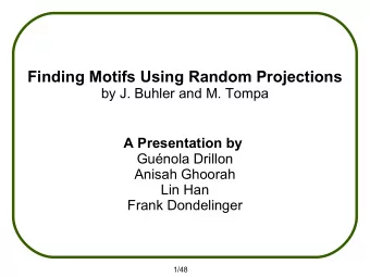
More Motifs WMM, log odds scores, Neyman-Pearson, background; - PowerPoint PPT Presentation

More Motifs WMM, log odds scores, Neyman-Pearson, background; Greedy & EM for motif discovery

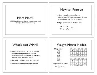
Neyman-Pearson • Given a sample x 1 , x 2 , ..., x n , from a distribution f(...| Θ ) with parameter Θ , want to test hypothesis Θ = θ 1 vs Θ = θ 2 . • Might as well look at likelihood ratio: f( x 1 , x 2 , ..., x n | θ 1 ) f( x 1 , x 2 , ..., x n | θ 2 ) > τ

What’s best WMM? • Given 20 sequences s 1 , s 2 , ..., s k of length 8, assumed to be generated at random according to a WMM defined by 8 x (4-1) parameters θ , what’s the best θ ? • E.g., what MLE for θ given data s 1 , s 2 , ..., s k ? • Answer: count frequencies per position.

Weight Matrix Models 8 Sequences: Freq. Col 1 Col 2 Col3 A .625 0 0 ATG C 0 0 0 ATG G .250 0 1 ATG ATG T .125 1 0 ATG GTG LLR Col 1 Col 2 Col 3 GTG - ∞ - ∞ A 1.32 TTG - ∞ - ∞ - ∞ C Log-Likelihood Ratio: - ∞ G 0 2.00 - ∞ T -1.00 2.00 f x i ,i , f x i = 1 log 2 f x i 4

Non-uniform Background • E. coli - DNA approximately 25% A, C, G, T • M. jannaschi - 68% A-T, 32% G-C LLR from previous LLR Col 1 Col 2 Col 3 example, assuming - ∞ - ∞ A .74 - ∞ - ∞ - ∞ C f A = f T = 3 / 8 - ∞ G 1.00 3.00 f C = f G = 1 / 8 - ∞ T -1.58 1.42 e.g., G in col 3 is 8 x more likely via WMM than background, so (log 2 ) score = 3 (bits).

WMM: How “Informative”? Mean score of site vs bkg? • For any fixed length sequence x , let P(x) = Prob. of x according to WMM Q(x) = Prob. of x according to background • Recall Relative Entropy: P ( x ) � H ( P || Q ) = P ( x ) log 2 Q ( x ) x ∈ Ω -H(Q||P) H(P||Q) • H(P||Q) is expected log likelihood score of a sequence randomly chosen from WMM ; -H(Q||P) is expected score of Background

For WMM, you can show (based on the assumption of independence between columns), that : H ( P || Q ) = � i H ( P i || Q i ) where P i and Q i are the WMM/background distributions for column i.

WMM Example, cont. Freq. Col 1 Col 2 Col3 A .625 0 0 C 0 0 0 G .250 0 1 T .125 1 0 Uniform Non-uniform LLR Col 1 Col 2 Col 3 LLR Col 1 Col 2 Col 3 - ∞ - ∞ - ∞ - ∞ A 1.32 A .74 - ∞ - ∞ - ∞ - ∞ - ∞ - ∞ C C - ∞ - ∞ G 0 2.00 G 1.00 3.00 - ∞ - ∞ T -1.00 2.00 T -1.58 1.42 RelEnt .70 2.00 2.00 4.70 RelEnt .51 1.42 3.00 4.93

Pseudocounts • Are the - ∞ ’s a problem? • Certain that a given residue never occurs in a given position? Then - ∞ just right • Else, it may be a small-sample artifact • Typical fix: add a pseudocount to each observed count—small constant (e.g., .5, 1) • Sounds ad hoc ; there is a Bayesian justification

How-to Questions • Given aligned motif instances, build model? • Frequency counts (above, maybe with pseudocounts) • Given a model, find (probable) instances? • Scanning, as above • Given unaligned strings thought to contain a motif, find it? (e.g., upstream regions for co- expressed genes from a microarray experiment) • Hard... next few lectures.

Motif Discovery: 3 example approaches • Greedy search • Expectation Maximization • Gibbs sampler Note: finding a site of max relative entropy in a set of unaligned sequences is NP-hard (Akutsu)

Greedy Best-First Approach [Hertz & Stormo] Input: usual “greedy” problems • Sequence s 1 , s 2 , ..., s k ; motif length I ; “breadth” d Algorithm: • create singleton set with each length l subsequence of each s 1 , s 2 , ..., s k • for each set, add each possible length l subsequence not already present • compute relative entropy of each • discard all but d best • repeat until all have k sequences

Expectation Maximization [MEME, Bailey & Elkan, 1995] Input (as above): • Sequence s 1 , s 2 , ..., s k ; motif length l ; background model; again assume one instance per sequence (variants possible) Algorithm: EM • Visible data: the sequences • Hidden data: where’s the motif � 1 if motif in sequence i begins at position j Y i,j = 0 otherwise • Parameters θ : The WMM

MEME Outline Typical EM algorithm: • Given parameters θ t at t th iteration, use them to estimate where the motif instances are (the hidden variables) • Use those estimates to re-estimate the parameters θ to maximize likelihood of observed data, giving θ t+1 • Repeat

Expectation Step (where are the motif instances?) ) 1 ( P 1 + · ) 0 ( P � 0 E ( Y i,j | s i , θ t ) = · = Y i,j E Bayes P ( Y i,j = 1 | s i , θ t ) = P ( s i | Y i,j = 1 , θ t ) P ( Y i,j =1 | θ t ) = P ( s i | θ t ) cP ( s i | Y i,j = 1 , θ t ) = � Y i,j c � � l k =1 P ( s i,j + k − 1 | θ t ) = where c � is chosen so that � 1 3 5 7 9 11 ... j � Sequence i Y i,j = 1.

Maximization Step (what is the motif?) Find θ maximizing expected value: Q ( θ | θ t ) = E Y ∼ θ t [log P ( s, Y | θ )] E Y ∼ θ t [log � k = i =1 P ( s i , Y i | θ )] E Y ∼ θ t [ � k = i =1 log P ( s i , Y i | θ )] E Y ∼ θ t [ � k � | s i | − l +1 = Y i,j log P ( s i , Y i,j = 1 | θ )] i =1 j =1 E Y ∼ θ t [ � k � | s i | − l +1 = Y i,j log( P ( s i | Y i,j = 1 , θ ) P ( Y i,j = 1 | θ ))] i =1 j =1 � k � | s i | − l +1 = E Y ∼ θ t [ Y i,j ] log P ( s i | Y i,j = 1 , θ ) + C i =1 j =1 � k � | s i | − l +1 � = Y i,j log P ( s i | Y i,j = 1 , θ ) + C i =1 j =1

M-Step (cont.) � k � | s i | − l +1 � Q ( θ | θ t ) = Y i,j log P ( s i | Y i,j = 1 , θ ) + C i =1 j =1 Exercise: Show this is s 1 : ACGGATT. . . maximized by “counting” . . . s k : GC. . . TCGGAC letter frequencies over all possible motif � ACGG Y 1 , 1 � instances, with counts CGGA Y 1 , 2 � GGAT Y 1 , 3 weighted by , again � Y i,j . . the “obvious” thing. . . . . � CGGA Y k,l − 1 � GGAC Y k,l

Initialization 1. Try every motif-length substring, and use as initial θ a WMM with, say 80% of weight on that sequence, rest uniform 2. Run a few iterations of each 3. Run best few to convergence (Having a supercomputer helps)